Plot time-varying PTE measures and treatment effects from a "fitted_onlinesurr" object
Source: R/methods.R
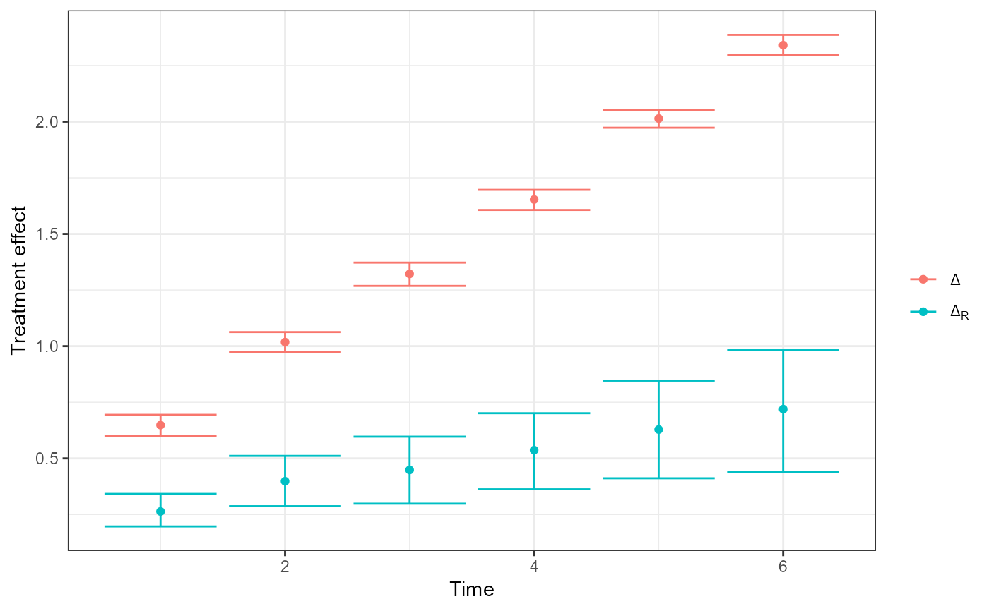
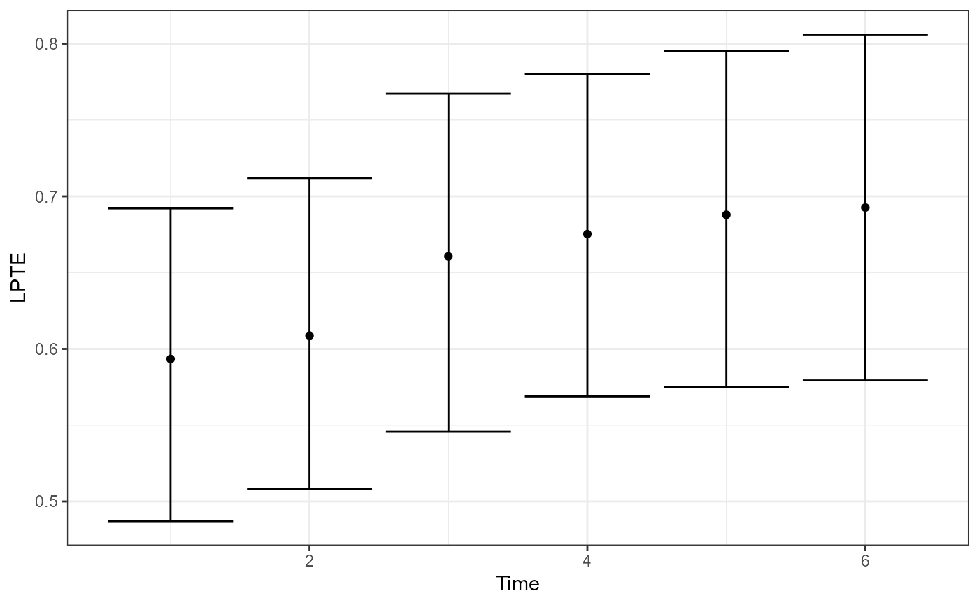
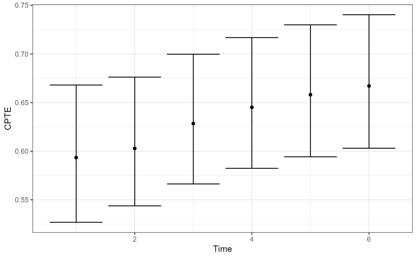
plot.fitted_onlinesurr.RdProduces a ggplot2 figure showing, over time, either the Local PTE (LPTE), the Cumulative PTE (CPTE), or the marginal and residual treatment effects \(\Delta(t)\) and \(\Delta_R(t)\) (labeled \(\Delta\) and \(\Delta_R\) in the plot). Point estimates are taken from object$Marginal$point and object$Conditional$point, with uncertainty bands computed from the stored bootstrap draws.
Usage
# S3 method for class 'fitted_onlinesurr'
plot(x, type = "LPTE", conf.level = 0.95, one.sided = TRUE, ...)
Arguments
- x
A
"fitted_onlinesurr"object, typically returned byfit.surr. It must contain$T,$n.fixed, and the components$Marginaland$Conditional, each withpointandsmp.- type
Character string specifying what to plot. One of
"LPTE","CPTE", or"Delta"(case-insensitive)."Delta"plots both \(\Delta(t)\) and \(\Delta_R(t)\) with separate colors.- conf.level
Numeric in \((0,1)\) giving the confidence level for the plotted intervals. Default is
0.95.- one.sided
Logical; if
TRUE(default), usessignif.level = (1-conf.level)/2when taking quantiles, so each tail excludes1-conf.level(i.e., a wider interval than the usual two-sidedconf.levelinterval). This is convenient when visually assessing one-sided surrogate validation criteria. IfFALSE, uses the standard two-sided constructionsignif.level = 1-conf.level.- ...
Additional arguments (currently unused) included for S3 method compatibility.
Details
The function extracts time-indexed treatment-effect estimates \(\Delta(t)\) (marginal) and \(\Delta_R(t)\) (residual/conditional) from the fitted object, along with bootstrap draws for each. It then constructs:
LPTE: \(\mathrm{LPTE}(t) = 1 - \Delta_R(t)/\Delta(t)\).
CPTE: \(\mathrm{CPTE}(t) = 1 - \sum_{u\le t}\Delta_R(u)/\sum_{u\le t}\Delta(u)\).
Delta: plots \(\Delta(t)\) and \(\Delta_R(t)\) directly.
Point estimates are plotted as points; intervals are empirical quantile intervals computed from the bootstrap sample matrices stored in object.
Examples
fit <- fit.surr(y ~ 1,
  id = id,
  surrogate = ~s,
  treat = trt,
  data = sim_onlinesurr, # This dataset is included in the OnlineSurr package
  time = time,
  verbose = 0,
  N.boots = 500 # Generally, this value would be too small.
  # Remember to increase it for your dataset.
)

plot(fit, type = "LPTE")

plot(fit, type = "CPTE", conf.level = 0.90, one.sided = FALSE)

plot(fit, type = "Delta")