Creates an outcome with Multinomial distribution with the chosen parameters.
Usage
Multinom(p, data, offset = as.matrix(data)^0, base.class = NULL)Arguments
- p
character: a vector with the name of the linear predictor associated with the probability of each category (except the base one, which is assumed to be the last).
- data
vector: Values of the observed data.
- offset
vector: The offset at each observation. Must have the same shape as data.
- base.class
character or integer: The name or index of the base class. Default is to use the last column of data.
Details
For evaluating the posterior parameters, we use the method proposed in Alves et al. (2024) .
For the details about the implementation see dos Santos et al. (2024) .
References
Mariane
Branco Alves, Helio
S. Migon, Raíra Marotta, Junior,
Silvaneo
Vieira dos Santos (2024).
“k-parametric Dynamic Generalized Linear Models: a sequential approach via Information Geometry.”
2201.05387.
Junior,
Silvaneo
Vieira dos Santos, Mariane
Branco Alves, Helio
S. Migon (2024).
“kDGLM: an R package for Bayesian analysis of Dynamic Generialized Linear Models.”
See also
Other auxiliary functions for a creating outcomes:
Gamma(),
Normal(),
Poisson(),
summary.dlm_distr()
Examples
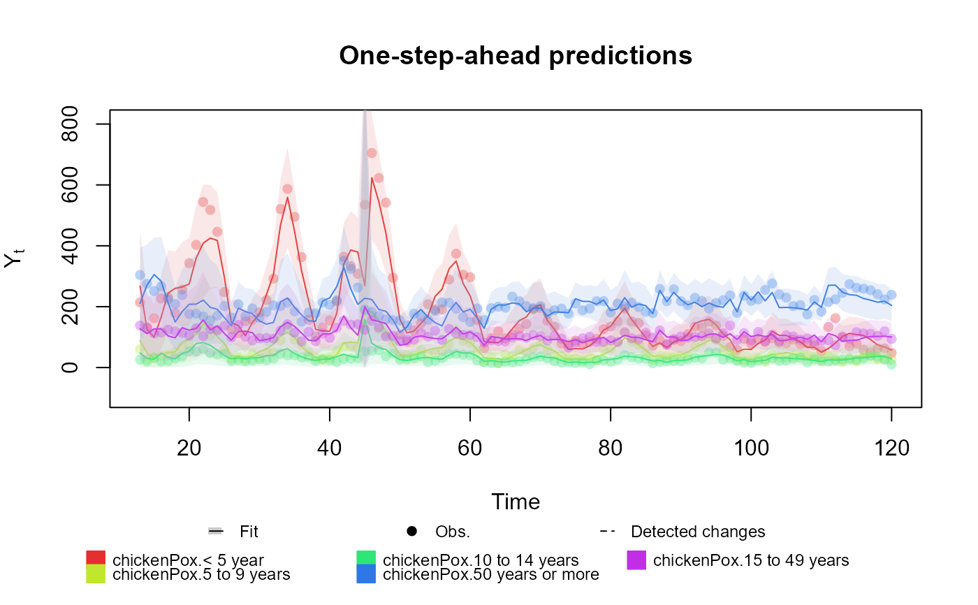
structure <- (
  polynomial_block(p = 1, order = 2, D = 0.95) +
    harmonic_block(p = 1, period = 12, D = 0.975) +
    noise_block(p = 1, R1 = 0.1) +
    regression_block(p = chickenPox$date >= as.Date("2013-09-01"))
  # Vaccine was introduced in September of 2013
) * 4

outcome <- Multinom(p = structure$pred.names, data = chickenPox[, c(2, 3, 4, 6, 5)])
fitted.data <- fit_model(structure, chickenPox = outcome)
summary(fitted.data)
#> Fitted DGLM with 1 outcomes.
#>
#> distributions:
#>     chickenPox: Multinomial
#>
#> Static coeficients (smoothed):
#>                  Estimate Std. Error   t value Pr(>|t|)
#> Var.Reg.1         0.39743    0.25059  1.58601    0.113
#> Var.Reg.2         0.47441    0.26448  1.79376    0.073 .
#> Var.Reg.3         0.48811    0.28497  1.71284    0.087 .
#> Var.Reg.4        -0.26900    0.23557 -1.14192    0.253
#> ---
#> Signif. codes:  0 ‘***’ 0.001 ‘**’ 0.01 ‘*’ 0.05 ‘.’ 0.1 ‘ ’ 1
#>
#> ---
#> See the coef.fitted_dlm for the coeficients with temporal dynamic.
#>
#> One-step-ahead prediction
#> Log-likelihood        : -1952.613
#> Interval Score        : 165.55741
#> Mean Abs. Scaled Error:   0.77058
#> ---
plot(fitted.data, plot.pkg = "base")