Introduction

This vignette is intended as an introduction to the usage of the kDGLM package, which offers routines for Bayesian analysis of Dynamic Generalized Linear Models, including fitting (filtering and smoothing), forecasting, sampling, intervention and automated monitoring, following the theory developed and/or explored in Kalman (1960), West and Harrison (1997) and Alves et al. (2024).

In this document we will focus exclusively in the usage of the package and will only briefly mention the theory behind these models and only with the intention of highlighting the notation. We highly recommend all users to read the theoretical work (dos Santos et al., 2024) in which we based this package.

This document is organized in the following order:

First we introduce the notations and the class of models we will be dealing with;
Next we present the details about the specification of the model structure, offering tools that allow for an easy, fast and (hopefully) intuitive way of defining models;
In the following section we discuss details about how the user can specify the observational model;
Then we present some basic examples of model fitting, also showing the auxiliary functions that help the user to analyse the fitted model. We also show tools for easy model selection;
Lastly, we present a variety of advanced examples, combining the basic features shown in previous sections to create more complex models;

Notation

In this section, we assume the user’s interest lies in analyzing a Time Series $\{\vec{Y}_t\}_{t=1}^T$ , which adheres to the model described by :

$\begin{equation} \begin{aligned} \vec{Y}_t|\vec{\eta}_t &\sim \mathcal{F}\left(\vec{\eta}_t\right),\\ g(\vec{\eta}_t) &=\vec{\lambda}_{t}=F_t'\vec{\theta}_t,\\ \vec{\theta}_t&=G_t\vec{\theta}_{t-1}+\vec{\omega}_t,\\ \vec{\omega}_t &\sim \mathcal{N}_n(\vec{h}_t,W_t), \end{aligned} \end{equation}$

The model comprises:

$\vec{Y}_t=(Y_{1,t},...,Y_{r,t})'$ , the outcome, is an $r$ -dimensional vector of observed variable.
$\vec{\theta}_t=(\theta_{1,t},...,\theta_{n,t})'$ , representing the unknown parameters (latent states), is an $n$ -dimensional vector, consistently dimensioned across observations.
$\vec{\lambda}_t=(\lambda_{1,t},...,\lambda_{k,t})'$ , the linear predictors, is a $k$ -dimensional vector indicating the linear transformation of the latent states. As per , $\vec{\lambda}_t$ is assumed to be (approximately) Normally distributed at all times and directly corresponds to the observational parameters $\vec{\eta}_t$ , through a one-to-one correspondence $g$ .
$\vec{\eta}_t=(\eta_{1,t},...,\eta_{l,t})'$ , the observational parameters, is an $l$ -dimensional vector defining the model’s observational aspects. Typically, $l=k$ , but this may not hold in some special cases, such as in the Multinomial model, where $k=l-1$ .
$\mathcal{F}$ , a distribution from the Exponential Family indexed by $\vec{\eta}_t$ . Pre-determines the values $k$ and $l$ , along with the link function $g$ .
$g$ , the link function, establishes a one-to-one correspondence between $\vec{\lambda}_t$ and $\vec{\eta}_t$ .
$F_t$ , the design matrix, is a user-defined, mostly known, matrix of size $k \times n$ .
$G_t$ , the evolution matrix, is a user-defined, mostly known, matrix of size $n \times n$ .
$\vec{h}_t=(h_{1,t},...,h_{n,t})'$ , the drift, is a known $n$ -dimensional vector, typically set to $\vec{0}$ except for model interventions (refer to subsection ).
$W_t$ , a known covariance matrix of size $n \times n$ , is specified by the user.

Per , we define $\mathcal{D}_t$ as the cumulative information after observing the first $t$ data points, with $\mathcal{D}_0$ denoting pre-observation knowledge of the process $\{Y_t\}^T_{t=1}$ .

The specification of $W_t$ follows , section 6.3, where $W_t=Var[G_t\theta_{t-1}|\mathcal{D}_{t-1}] \odot (1-D_t) \oslash D_t + H_t$ . Here, $D_t$ (the discount matrix) is an $n \times n$ matrix with values between $0$ and $1$ , $\odot$ represents the Hadamard product, and $\oslash$ signifies Hadamard division. $H_t$ is another known $n \times n$ matrix specified by the user. This formulation implies that if $D_t$ entries are all $1$ , and $H_t$ entries are all $0$ , the model equates to a Generalized Linear Model.

A prototypical example within the general model framework is the Poisson model augmented with a dynamic level featuring linear growth and a single covariate $X$ :

$\begin{equation} \begin{aligned} Y_t|\eta_t &\sim \mathcal{P}\left(\eta_t\right),\\ ln(\eta_t) &=\lambda_{t}=\mu_t+\beta_t X_t,\\ \mu_t&=\mu_{t-1}+\beta_{t-1}+\omega_{\mu,t},\\ \nu_t&=\nu_{t-1}+\omega_{\nu,t},\\ \beta_t&=\beta_{t-1}+\omega_{\beta,t},\\ \omega_{\mu,t},\omega_{\nu,t},\omega_{\beta,t} &\sim \mathcal{N}_3(\vec{0},W_t), \end{aligned} \end{equation}$

In this model, $\mathcal{F}$ denotes the Poisson distribution; the model dimensions are $r=k=l=1$ ; the state vector $\theta_t$ is $(\mu_t,\nu_t,\beta_t)'$ with dimension $n=3$ ; the link function $g$ is the natural logarithm; and the matrices $F_t$ and $G_t$ are defined as:

$F_t=\begin{bmatrix} 1 \\ 0 \\ X_t \end{bmatrix} \quad G_t=\begin{bmatrix} 1 & 1 & 0 \\ 0 & 1 & 0 \\ 0 & 0 & 1 \end{bmatrix}$

Consider now a Normal model with unknown mean $\eta_{1,t}$ and unknown precision $\eta_{2,t}$ :

$\begin{equation} \begin{aligned} Y_t|\eta_t &\sim \mathcal{N}\left(\eta_{1,t},\eta_{2,t}^{-1}\right),\\ \eta_{1,t} &=\lambda_{1,t}=\mu_{1,t}+\beta_t X_t,\\ ln(\eta_{2,t}) &=\lambda_{2,t}=\mu_{2,t},\\ \mu_{1,t}&=\mu_{1,t-1}+\beta_{t-1}+\omega_{\mu_1,t},\\ \nu_t&=\nu_{t-1}+\omega_{\nu,t},\\ \beta_t&=\beta_{t-1}+\omega_{\beta,t},\\ \mu_{2,t}&=\phi_{t-1}\mu_{2,t-1}+\omega_{\mu_2,t},\\ \phi_{t}&=\phi_{t-1}+\omega_{\phi,t},\\ \omega_{\mu_1,t},\omega_{\nu,t},\omega_{\mu,t},\omega_{\beta,t},\omega_{\phi,t} &\sim \mathcal{N}_5(\vec{0},W_t), \end{aligned} \end{equation}$

For this case, $\mathcal{F}$ represents the Normal distribution; the model dimensions are $r=1$ and $k=l=2$ ; the state vector $\theta_t$ is $(\mu_{1,t},\nu_t,\beta_t,\mu_{2,t},\phi_t)'$ with dimension $n=5$ ; the link function $g$ and matrices $F_t$ , $G_t$ are:

$g\left(\begin{bmatrix} x_1 \\ x_2 \end{bmatrix}\right)= \begin{bmatrix} x_1 \\ \ln(x_2) \end{bmatrix}\quad F_t=\begin{bmatrix} 1 & 0 \\ 0 & 0\\ X_t & 0 \\ 0 & 1 \\ 0 & 0 \end{bmatrix} \quad G_t=\begin{bmatrix} 1 & 1 & 0 & 0 & 0\\ 0 & 1 & 0 & 0 & 0\\ 0 & 0 & 1 & 0 & 0\\ 0 & 0¨& 0 & \phi & 0\\ 0 & 0¨& 0 & 0 & 1 \end{bmatrix}$

This configuration introduces $l=2$ observational parameters, necessitating $k=2$ linear predictors. The first linear predictor pertains to the location parameter of the Normal distribution and includes a linear growth model and the covariate $X_t$ . The second linear predictor, associated with the precision parameter, models log precision as an autoregressive (AR) process. We express this model in terms of an Extended Kalman Filter (Kalman, 1960; West and Harrison, 1997). This formulation aligns with the concept of a traditional Stochastic Volatility model, as highlighted by Alves et al. (2024).

Both the Normal and Poisson models illustrate univariate cases. However, the general model also accommodates multivariate outcomes, such as in the multinomial case. Consider a vector of counts $\vec{Y}_t=(Y_{1,t},Y_{2,t},Y_{3,t},Y_{4,t},Y_{5,t})'$ , with $Y_{i,T} \in \mathbb{Z}$ and $N_t=\sum_{i=1}^{5}Y_{i,t}$ . The model is:

$\begin{equation} \begin{aligned} \vec{Y}_{5,t}|N_t,\vec{\eta}_{t} &\sim Multinomial\left(N_t,\vec{\eta}_{t}\right),\\ \ln\left(\frac{\eta_{i,t}}{\eta_{5,t}}\right) &=\lambda_{1,t}=\mu_{i,t},i=1,...,4\\ \mu_{i,t}&=\mu_{i,t-1}+\omega_{\mu_i,t},i=1,...,4\\ \omega_{\mu_1,t},\omega_{\mu_2,t},\omega_{\mu_3,t},\omega_{\mu_4,t} &\sim \mathcal{N}_4(\vec{0},W_t), \end{aligned} \end{equation}$

In this multinomial model, $\mathcal{F}$ is the Multinomial distribution; the model dimensions are $r=5$ , $l=5$ and $k=4$ ; the state vector $\theta_t$ is $(\mu_{1,t},\mu_{2,t},\mu_{3,t},\mu_{4,t})'$ ; $F_t$ and $G_t$ are identity matrices of size $4\times 4$ ; and the link function $g$ maps $\mathbb{R}^5$ in $\mathbb{R}^{4}$ as:

$g\left(\begin{bmatrix} x_1 \\ x_2 \\ x_3 \\ x_4 \\ x_5 \end{bmatrix}\right)= \begin{bmatrix} \ln\left(\frac{x_1}{x_5}\right) \\ \ln\left(\frac{x_2}{x_5}\right) \\ \ln\left(\frac{x_3}{x_5}\right) \\ \ln\left(\frac{x_4}{x_5}\right) \end{bmatrix}$

Note that in the Multinomial distribuition, $\eta_i\ge 0, \forall i$ and $\sum_{i=1}^{5} \eta_i=1$ . Thus, only $k=l-1$ linear predictors are necessary to describe this model.

It’s important to emphasize that while we have chosen to illustrate simple model structures, such as a random walk in the log odds for each outcome, neither the general model framework nor the kDGLM package restricts to these configurations. Analysts have the flexibility to tailor models to their specific contexts, including the incorporation of additional latent states to enhance outcome explanation.

Lastly, this general model framework can be extended to encompass multiple outcome models. For further details, see Handling multiple outcomes.

Given the complexity of manually specifying all model components, the kDGLM package includes a range of auxiliary functions to simplify this process. The subsequent section delves into these tools.

Single outcome models

The kDGLM package supports the joint modelling of multiple time series, each with it own structure and distribution (see Handling multiple outcomes). This flexibility comes with a somewhat complex syntax, designed to allow analysts to meticulously define every aspect of the model. While we have aimed to create an intuitive yet powerful syntax, we recognize that it may feel overwhelming for new users. To address this, the kDGLM package also provides a simplified syntax, similar to the lm and glm functions native to R. This simplified approach supports single-outcome models with any of the supported distributions, while still allowing for complex dynamic structures in all parameters of the observational distribution.

Lets consider the classic airline data, which is comprised of monthly totals of international airline passengers, from 1949 to 1960. We can adjust a simple Time Series model using the following code:

fitted.data <- kdglm(c(AirPassengers) ~ 1, family = Poisson)
plot(fitted.data)

Detail about the plot method can be found in Filtering and smoothing, for now we focus only on the usage of the kdglm function. By the default, the intercept of a model is considered dynamic in a discount factor of $0.95$ . One can specify the details of the intercept using the pol function inside the formula:

fitted.data <- kdglm(c(AirPassengers) ~ pol(D = 0.99), family = Poisson)
plot(fitted.data)

One can also add more complex structures to the model using the functions $har$ , $reg$ , $AR$ , $TF$ and $noise$ :

fitted.data <- kdglm(c(AirPassengers) ~ pol(D = 0.99, order = 2) + har(period = 12) + noise(R1 = 0.01), family = Poisson)
plot(fitted.data)

For more details, see Structures.

For dynamic regressions, the kdglm package adopts the same convetions as the lm and glm functions:

# Total number of cases
chickenPox$Total <- rowSums(chickenPox[, c(2, 3, 4, 6, 5)])
# Indicator of the introcution of the chicken pox vaccine to the national program of immunization
chickenPox$Vaccine <- chickenPox$date >= as.Date("2013-09-01")

fitted.data <- kdglm(`< 5 year` ~ pol(2, D = 0.95) + har(12, D = 0.975) + Vaccine,
  N = chickenPox$Total,
  family = Multinom,
  data = chickenPox
)
plot(fitted.data, plot.pkg = "base")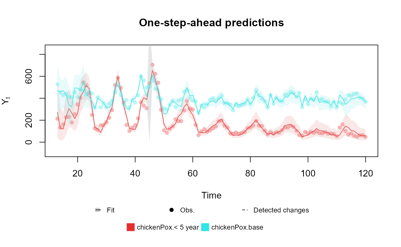

For the multinomial case, where we the outcome of the model is a vector, the user may include several formulas, one for each index of the outcome vector:

fitted.data <- kdglm(
  `< 5 year` ~ pol(2, D = 0.95) + har(12, D = 0.975) + Vaccine,
  `10 to 14 years` ~ pol(2, D = 0.95) + har(12, D = 0.975) + Vaccine,
  `15 to 49 years` ~ pol(2, D = 0.95) + har(12, D = 0.975) + Vaccine,
  `50 years or more` ~ pol(2, D = 0.95) + har(12, D = 0.975) + Vaccine,
  N = chickenPox$Total,
  family = Multinom,
  data = chickenPox
)
plot(fitted.data, plot.pkg = "base")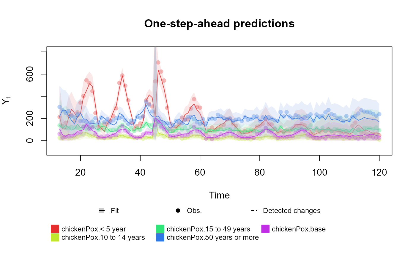

Lastly, some outcomes may require extra arguments for the parameters of the observational model. For instance, the kdglm package allows for dynamic structure for all parameters of a model, so for the Normal family, the user may include dynamic structure for both mean and variance:

fitted.data <- kdglm(corn.log.return ~ 1,
  V = ~1,
  family = Normal,
  data = cornWheat[1:500, ]
)
plot(fitted.data, plot.pkg = "base")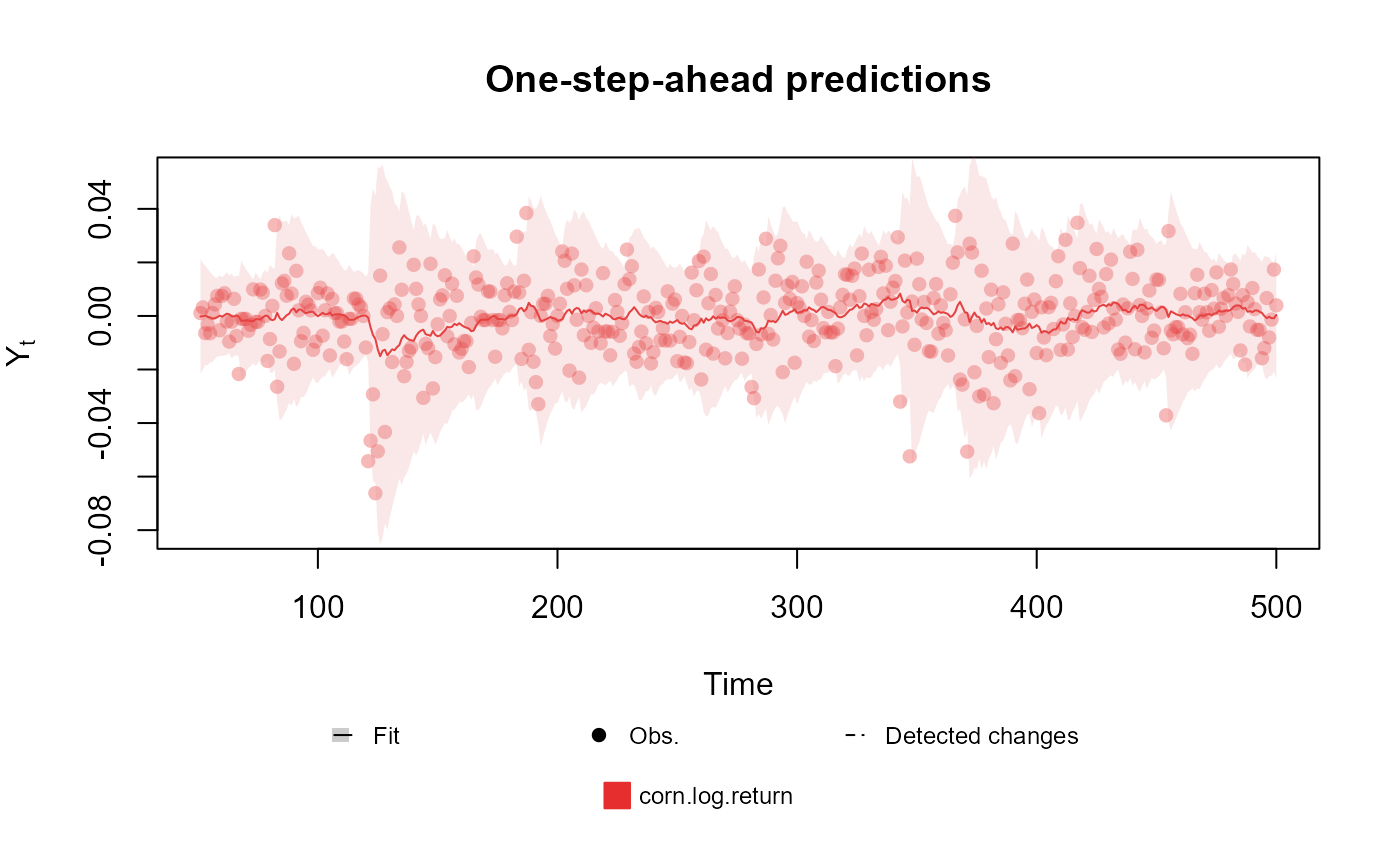

For more details about each outcome see Outcomes.

References

Alves, M. B., Migon, H. S., Marotta, R., and dos Santos, S. V., Junior. (2024). K-parametric dynamic generalized linear models: A sequential approach via information geometry.

dos Santos, S. V., Junior, Alves, M. B., and Migon, H. S. (2024). kDGLM: An r package for bayesian analysis of dynamic generialized linear models.

Kalman, R. E. (1960). A new approach to linear filtering and prediction problems. Transactions of the ASME–Journal of Basic Engineering, 82(Series D), 35–45.

West, M., and Harrison, J. (1997). Bayesian forecasting and dynamic models (springer series in statistics). Hardcover; Springer-Verlag.

Introduction

Table of contents

Introduction

Notation

Single outcome models

References