Fit a model given its structure and the observed data. This function can be used for any supported family (see vignette).
Arguments
- formula
an object of class "formula" (or one that can be coerced to that class): a symbolic description of the model to be fitted.
- ...
Extra arguments, including extra formulas (multinomial case) or extra parameters (normal and gamma cases).
- family
a description of the error distribution to be used in the model. For kdglm this can be a character string naming a family function or a family function.
- data
an optional data frame, list or environment (or object coercible by as.data.frame to a data frame) containing the variables in the model. If not found in data, the variables are taken from environment(formula), typically the environment from which glm is called.
- offset
this can be used to specify an a priori known component to be included in the linear predictor during fitting. This should be NULL or a numeric vector of length equal to the number of cases. One or more offset terms can be included in the formula instead.
- p.monit
numeric (optional): The prior probability of changes in the latent space variables that are not part of its dynamic. Only used when performing sensitivity analysis.
Details
This is the main function of the kDGLM package, as it is used to fit all models.
For the details about the implementation see dos Santos et al. (2024) .
For the details about the methodology see Alves et al. (2024) .
For the details about the Dynamic Linear Models see West and Harrison (1997) and Petris et al. (2009) .
See also
auxiliary functions for creating outcomes Poisson, Multinom, Normal, Gamma
auxiliary functions for creating structural blocks polynomial_block, regression_block, harmonic_block, TF_block
auxiliary functions for defining priors zero_sum_prior, CAR_prior
Other auxiliary functions for fitted_dlm objects:
coef.fitted_dlm(),
eval_dlm_norm_const(),
fit_model(),
forecast.fitted_dlm(),
simulate.fitted_dlm(),
smoothing(),
update.fitted_dlm()
Examples
# Poisson case
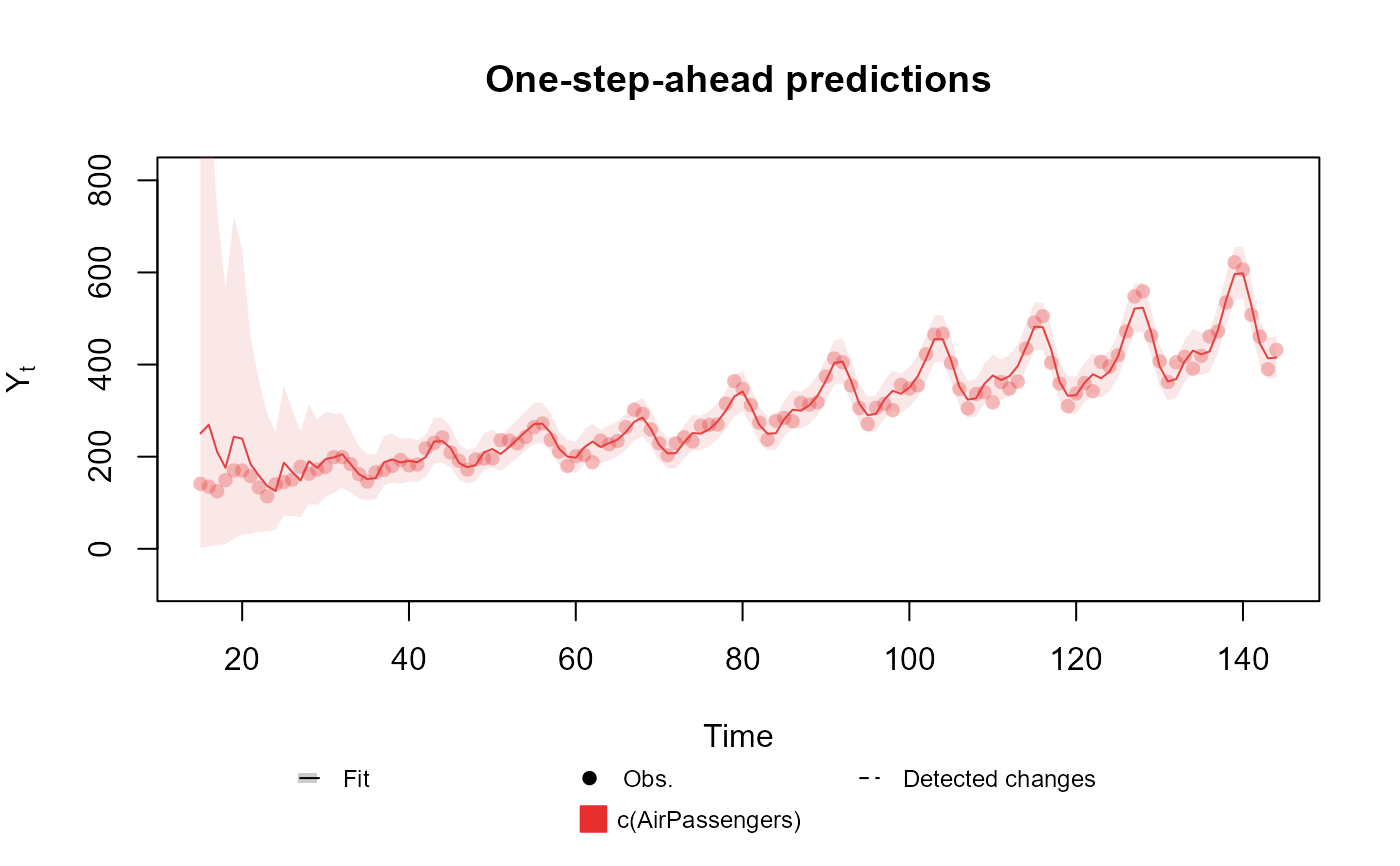
fitted.data <- kdglm(c(AirPassengers) ~ pol(2) + har(12, order = 2), family = Poisson)
summary(fitted.data)
#> Fitted DGLM with 1 outcomes.
#>
#> distributions:
#>     c(AirPassengers): Poisson
#>
#> ---
#> No static coeficients.
#> ---
#> See the coef.fitted_dlm for the coeficients with temporal dynamic.
#>
#> One-step-ahead prediction
#> Log-likelihood        : -582.8016
#> Interval Score        : 140.37692
#> Mean Abs. Scaled Error:   0.51246
#> ---
plot(fitted.data, plot.pkg = "base")


##################################################################

# Multinomial case
chickenPox$Total <- rowSums(chickenPox[, c(2, 3, 4, 6, 5)])
chickenPox$Vaccine <- chickenPox$date >= as.Date("2013-09-01")
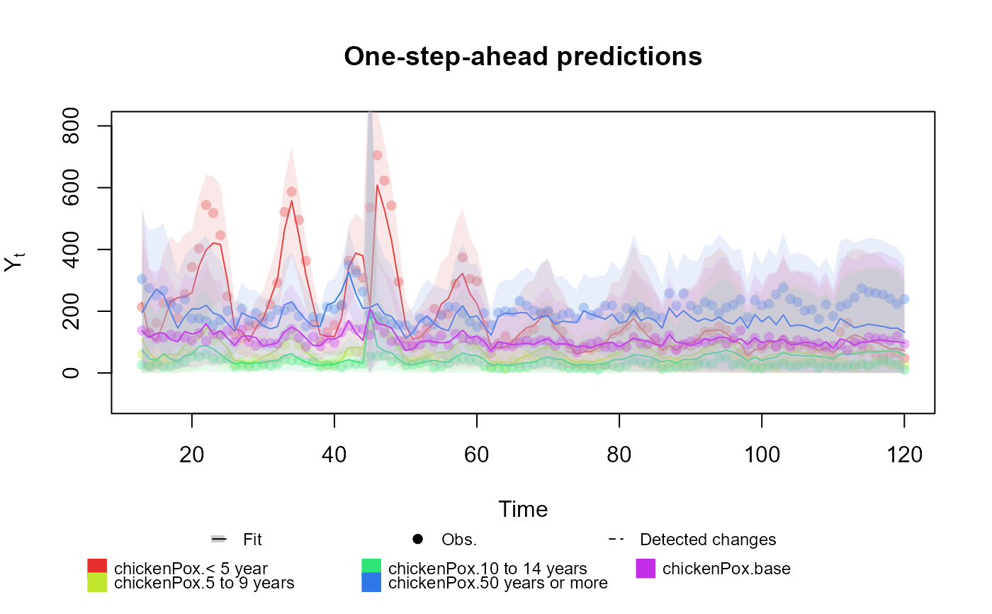
fitted.data <- kdglm(`< 5 year` ~ pol(2, D = 0.95) + har(12, D = 0.975) + noise(R1 = 0.1) + Vaccine,
  `5 to 9 years` ~ pol(2, D = 0.95) + har(12, D = 0.975) + noise(R1 = 0.1) + Vaccine,
  `10 to 14 years` ~ pol(2, D = 0.95) + har(12, D = 0.975) + noise(R1 = 0.1) + Vaccine,
  `50 years or more` ~ pol(2, D = 0.95) + har(12, D = 0.975) + noise(R1 = 0.1) + Vaccine,
  N = chickenPox$Total,
  family = Multinom,
  data = chickenPox
)
summary(fitted.data)
#> Fitted DGLM with 1 outcomes.
#>
#> distributions:
#>     chickenPox: Multinomial
#>
#> ---
#> No static coeficients.
#> ---
#> See the coef.fitted_dlm for the coeficients with temporal dynamic.
#>
#> One-step-ahead prediction
#> Log-likelihood        : -2169.169
#> Interval Score        :  255.27963
#> Mean Abs. Scaled Error:    1.24724
#> ---
plot(fitted.data, plot.pkg = "base")


##################################################################

# Univariate Normal case
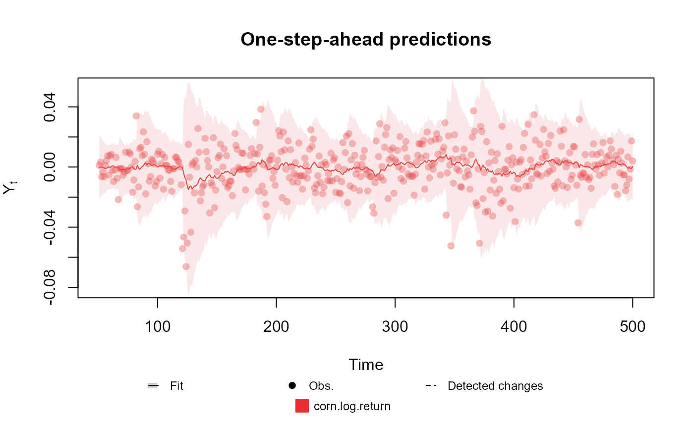
fitted.data <- kdglm(corn.log.return ~ 1, V = ~1, family = Normal, data = cornWheat[1:500, ])
summary(fitted.data)
#> Fitted DGLM with 1 outcomes.
#>
#> distributions:
#>     corn.log.return: Normal
#>
#> ---
#> No static coeficients.
#> ---
#> See the coef.fitted_dlm for the coeficients with temporal dynamic.
#>
#> One-step-ahead prediction
#> Log-likelihood        : 1277.54
#> Interval Score        : 0.07564
#> Mean Abs. Scaled Error: 0.76327
#> ---
plot(fitted.data, plot.pkg = "base")


##################################################################

# Gamma case
Y <- (cornWheat$corn.log.return[1:500] - mean(cornWheat$corn.log.return[1:500]))**2
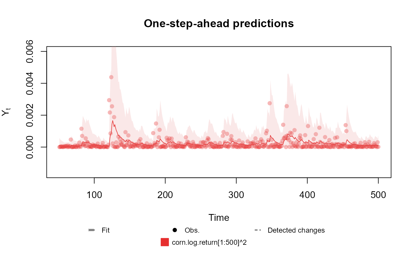
fitted.data <- kdglm(Y ~ 1, phi = 0.5, family = Gamma, data = cornWheat)
summary(fitted.data)
#> Fitted DGLM with 1 outcomes.
#>
#> distributions:
#>     Y: Gamma
#>
#> ---
#> No static coeficients.
#> ---
#> See the coef.fitted_dlm for the coeficients with temporal dynamic.
#>
#> One-step-ahead prediction
#> Log-likelihood        : 3508.409
#> Interval Score        : 0.00197
#> Mean Abs. Scaled Error: 0.93721
#> ---
plot(fitted.data, plot.pkg = "base")
