Fitting and analysing models

In this section we briefly present the usage of the fit_model function, along side the auxiliary functions for analyzing a fitted model, such as the summary, coef,plot, forecast and simulate methods. For a deep dive in the details of each argument of each function, see the documentation of those function and/or the reference manual.

Filtering and smoothing

The ... argument receives dlm_block and dlm_distr objects, the creation of which was described in the previous sections. In particular, if the user gives a dlm_distr object as a named argument, its name is used as the label for that outcome.

The argument smooth is a Boolean indicating if the smoothed distribution of the latent states should be evaluated. In general, we recommend the users to not change this value, as the computational cost of smoothing is usually negligible.

p_monit controls the sensitivity of the automated monitoring and we shall discuss its usage in subsection Intervention and monitoring.

Bellow we present a code that fits a Poisson model:

level <- polynomial_block(rate = 1, order = 2, D = 0.95)
season <- harmonic_block(rate = 1, period = 12, order = 2, D = 0.975)

outcome <- Poisson(lambda = "rate", data = c(AirPassengers))

fitted.model <- fit_model(
  level, season, # Strucuture
  AirPassengers = outcome
) # outcome

The first two lines create structural blocks representing a random walk on \(\mu_t\) and a seasonal component described by harmonics. The fourth line creates a Poisson outcome such that the rate parameter lambda is equal to \(\exp\{\text{rate}\}\), where rate is the label given to the linear predictor when creating the structural blocks (see section Creating the model structure for details about the linear predictor). The last line receives the model structure and the Poisson outcome and fits the model, obtaining the parameters for the filtered and smoothed distribution of all latent states.

The user can see how the model fits the data using the plot method, the syntax of which is as follows:

plot.fitted_dlm(model, pred.cred = 0.95, lag = 1, cutoff = floor(model$t / 10), plot.pkg = "auto")

The model argument must be a fitted_dlm object (i.e., the output of the fit_model function).

pred.cred must be a number between \(0\) and \(1\) representing the desired credibility of the predictions.

lag must be an integer representing the number of steps ahead to be used for predictions. If lag\(<0\), the smoothed distribution is used for predictions and, if lag\(=0\), the filtered distribution is used Instead.

cutoff must be an integer representing the number of initial steps that should be omitted in the plot. Usually, the model is still learning in the initial steps, so the predictions are not reliable. The default value is one tenth of the sample size rounded down.

Lastly plot.pkg must be a string specifying the plot engine to be used. Should be one of 'auto', 'base', 'ggplot2' or 'plotly'. If 'auto' is used, then the function tries to use the plotly package, if it fails, then it tries to use the ggplot2 packge and, if it also fails, the native functions provided by R will be used.

plot(fitted.model, plot.pkg = "base")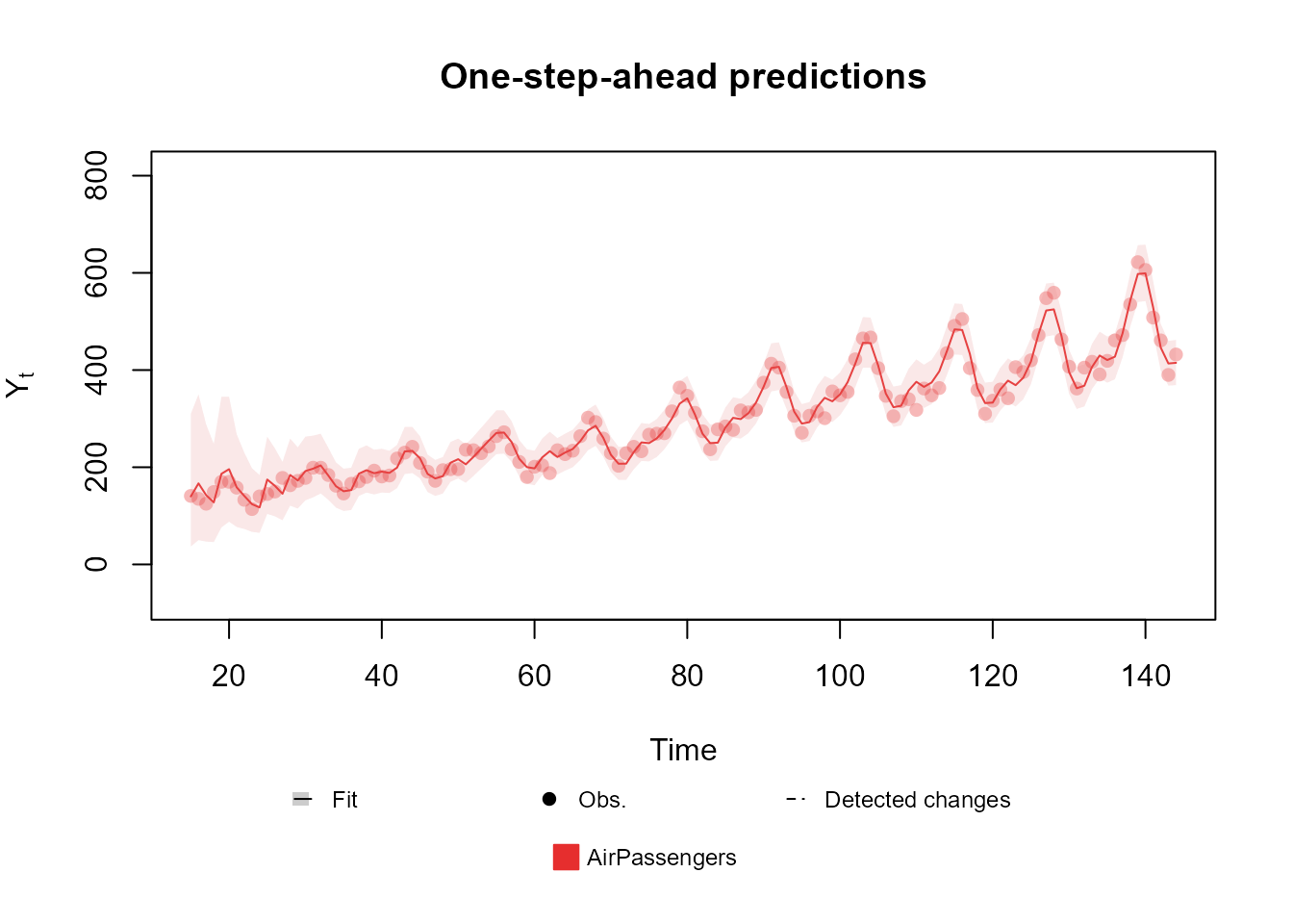

The remaining functions and methods in this section have similar usage as the plot.fitte_dlm method, as such, for the sake of brevity, we will only highlight the unique arguments and/or behaviors of each function or method present. We strongly advise the user to consult the reference manual and the documentation of each function for detailed descriptions of any function.

To see a summary of the fitted model, one can use the summary method:

summary(fitted.model)

Fitted DGLM with 1 outcomes.

distributions:
    AirPassengers: Poisson

---
No static coeficients.
---
See the coef.fitted_dlm for the coeficients with temporal dynamic.

One-step-ahead prediction
Log-likelihood        : -572.0896
Interval Score        : 106.83846
Mean Abs. Scaled Error:   0.40837
---

Note that only the static components of the model, i.e. those without temporal dynamic, were shown in the summary. This is so because is unpratical to show the values of all latent states at all times in the summary, while showing one specific time can lead to misleading results for unaware users. To see latent states with temporal dynamic, one must use the coef or plot methods.

For more details about the usage of the summary method, see the associated documentation (help(summary.fitted_dlm)).

Extracting components

Naturally, the user may want to extract information about the posterior distribution of the parameters of the fitted model, such that a more thorough analysis may be performed. For extracting the parameters of the distribution of latent states, linear predictors and observational model parameters, one can use the coef method:

coef(object, t.eval = seq_len(object$t), lag = -1, pred.cred = 0.95, eval.pred = FALSE, eval.metric = FALSE, ...)

The object parameter must be specified as a fitted_dlm object, which represents the model from which the components will be extracted. The t.eval parameter should be a vector that denotes the time indices at which the posterior is to be evaluated. The parameters lag and pred.cred retain their meanings analogous to those in the plot method of the fitted_dlm class. The eval.pred parameter requires a boolean value, indicating whether the predictive distribution for the observations is to be evaluated. Additionally, the eval.pred parameter should be a boolean specifying whether the model comparison metrics are to be computed.

The output of this function is a dlm_coef object containing:

data: A data frame with the model evaluated at each observed time.
mt: A \(n \times T\) matrix representing the mean of the latent states at each time, where \(n\) is the number of latent states in the model and \(T\) is the length of the time series;
Ct: A 3D-array containing the covariance matrix of the latent state at each time. Dimensions are \(n \times n \times T\);
ft: A \(k \times T\) matrix representing the mean of the linear predictor at each time, where \(k\) is the number of linear predictors in the model and \(T\) is the length of the time series;
Qt: A 3D-array containing the covariance matrix for the linear predictor at each time. Dimensions are \(k \times k \times T\);
Several vectors with some metrics, including the predictive log-likelihood, Mean Absolute Scaled Error (MASE, Hyndman and Koehler, 2006) and the Interval Score (interval.score, Bracher, 2021).
conj.param: A list containing the parameters for the conjugate distribution of the parameter of the observational model.

It is important to highlight that, following the method proposed in Alves et al. (2024), the joint distribution of the latent states and linear predictors at each time is Gaussian, such that the mean vector and covariance matrix completely define their distribution.

The user may also want to plot the latent states, for which the plot method for the dlm_coef class can be used:

fitted.coef <- coef(fitted.model)
plot(fitted.coef, plot.pkg = "base")

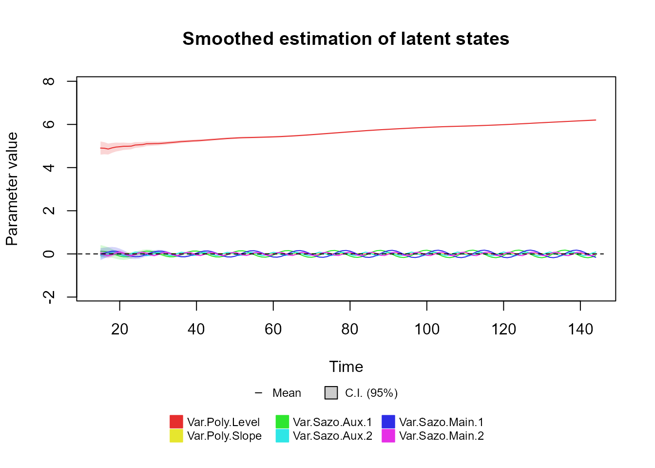
If the user wants to see only a restricted set of latent states, the extra argument var can be used to specify the label of the variables to plot:

plot(fitted.coef, "Var.Poly.Level", plot.pkg = "base")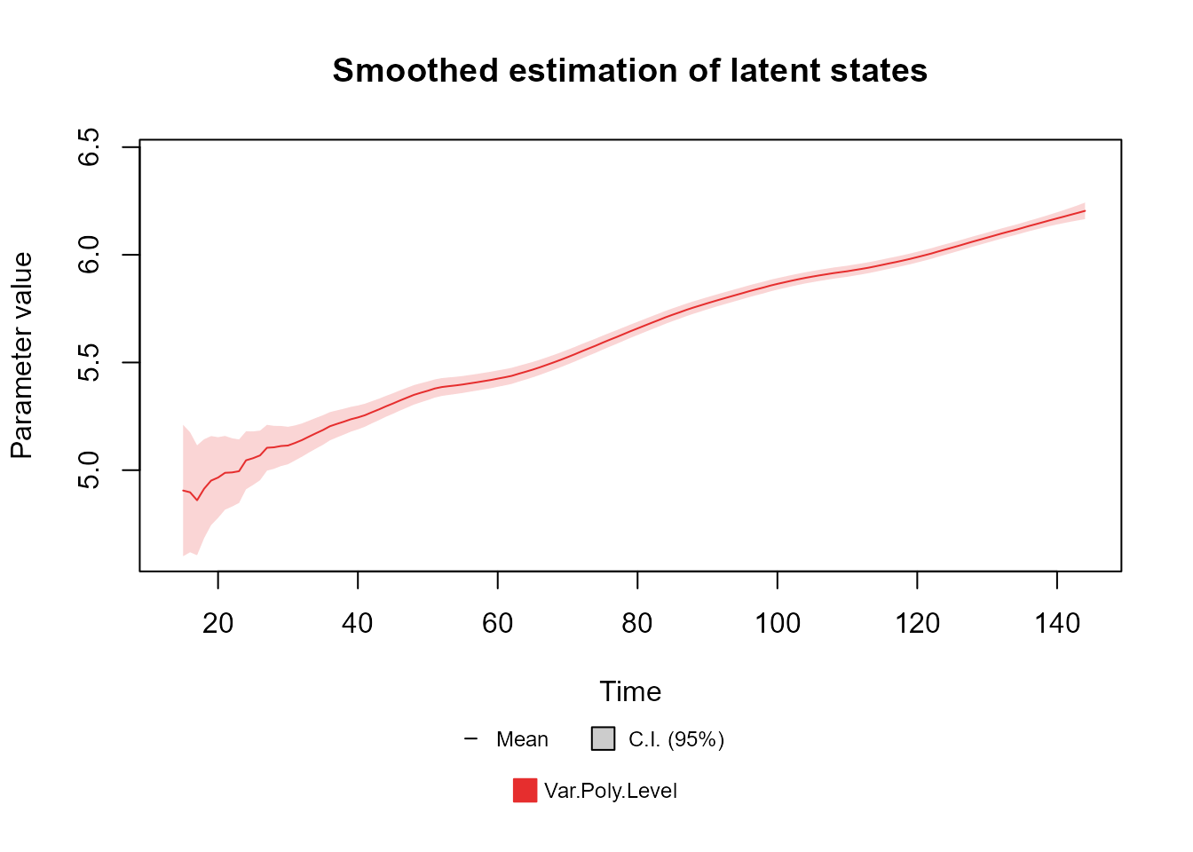

The user may also plot the linear predictors, by specifying the name of the linear predictor:

plot(fitted.coef, "rate", plot.pkg = "base")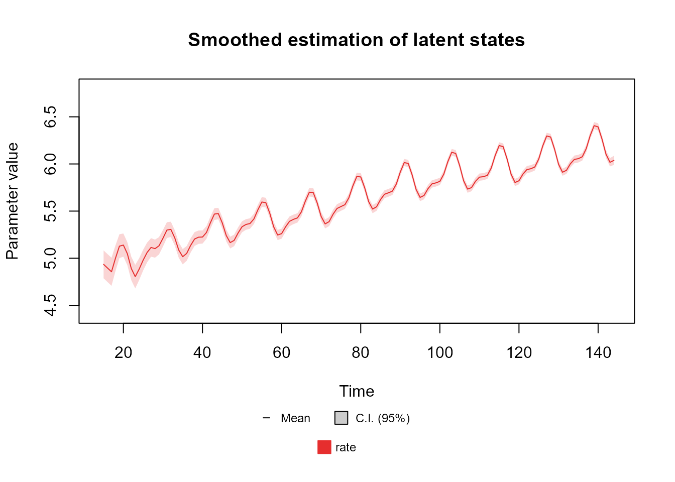

Lastly, although we do not recommend it, the user may also extract some of these information directly from the fitted_dlm object.

We strongly recommend every user to consult the documentation of each of these functions to see the full set of features provided by the kDGLM package.

Forecasting

Notice that all methods and functions presented previously were restricted to the period where the model was fitted. If the user wishes make predictions for future observations, the forecast method can be used:

forecast(object,
  t = 1,
  plot = ifelse(requireNamespace("plotly", quietly = TRUE), "plotly", ifelse(requireNamespace("ggplot2", quietly = TRUE), "ggplot2", "base")),
  pred.cred = 0.95,
  ...
)

The object parameter is required to be a fitted_dlm object. The t parameter specifies the prediction window. The plot parameter determines whether a plot should be generated and, if applicable, which engine to use, akin to the plot method in the fitted_dlm class. The pred.cred parameter signifies the credibility of the confidence intervals.

forecast(fitted.model, t = 20, plot = "base")$plot

Additionally to a plot (which is optional), the forecast method for the fitted_dlm class also provides a similar set of attributes of that which the dlm_coef class has, specifically, the predictive distribution for the latent states, the linear predictors and the observational model parameters, along with the predictions for future observations.

It is relevant to point out that if external data is necessary for forecasting, such as for models with regressive blocks or transfer functions, it is necessary to pass those values for the forecast method. In this scenario, the user must pass a new argument named as the variable that is “missing” from the model. See the documentation to see how to determine the name of the missing values or, more practically, try to use the forecast method without the necessary arguments, since the name of the missing variables will be presented in the error message.

Here we present two examples for a model with Multinomial outcome: One where the covariates where not properly passed and another where they were:

structure <-
  polynomial_block(p = 1, order = 2, D = 0.95) +
  harmonic_block(p = 1, period = 12, D = 0.975) +
  noise_block(p = 1, R1 = 0.1) +
  regression_block(
    p = chickenPox$date >= as.Date("2013-09-1"),
    # Vaccine was introduced in September of 2013
    name = "Vaccine"
  )

outcome <- Multinom(p = c("p.1", "p.2"), data = chickenPox[, c(2, 3, 5)])
fitted.model <- fit_model(structure * 2, chickenPox = outcome)

forecast(fitted.model, t = 24, plot = "base") # Missing extra arguments

Error in forecast.fitted_dlm(fitted.model, t = 24, plot = "base"): Error: Missing extra argument: Vaccine.1.Covariate

forecast(fitted.model,
  t = 24,
  Vaccine.1.Covariate = rep(TRUE, 24), # Extra argument for covariate 1
  Vaccine.2.Covariate = rep(TRUE, 24), plot = "base"
) # Extra argument for covariate 2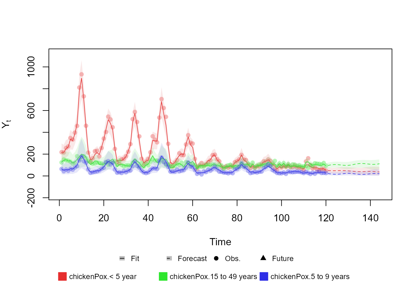

For more details on the usage of this function, see the associated documentation.

Updating a fitted model

One of the major advantages of the sequential nature of the methodology proposed in Alves et al. (2024) is that it allows for the updating of the posterior distribution of the parameter when new data arrives, but without the necessity of reprocessing the data previously observed. This feature is particularly useful in problems that involve monitoring or real time inference about a phenomena.

For updating a fitted_dlm object, the user can use the update method for the fitted_dlm class:

update.fitted_dlm(object, ...)

The object argument must be a fitted_dlm object. Moreover, the ... argument must be a sequence of named arguments containing the new information observed. For example:

level <- polynomial_block(rate = 1, order = 2, D = 0.95)
season <- harmonic_block(rate = 1, period = 12, order = 2, D = 0.975)
# Omitting the last 44 observations
outcome <- Poisson(lambda = "rate", data = c(AirPassengers)[1:100])
fitted.model <- fit_model(
  level, season, # Strucuture
  AirPassengers = outcome
) # outcome
updated.fit <- update(fitted.model,
  AirPassengers = list(data = c(AirPassengers)[101:144])
)

Note that the name of the argument containing the new observations must be the label given to that outcome when first fitting the model. In this case, the argument must be named update, as this was the label used in the fit_model function If a label was not provided when fitting the model, a default name will be used, which consist of the string 'Series.' followed by a proper index for that outcome.

The update function may require extra arguments containing covariates, pulses (for the transfer function), the offset, etc.. In such cases, the syntax is the same as the forecast method.

Intervention and monitoring

As a key feature, the kDGLM package has support for intervention and automated monitoring. First, if the user is aware that at some specific time there is some change in the time series that is not part of its temporal dynamic, then the user should provide that information in the model structure. For that we provide the intervention function:

data <- c(AirPassengers)
# Adding an artificial change, so that we can make an intervention on the data at that point
# Obviously, one should NOT change their own data.
data[60:144] <- data[60:144] + 100

level <- polynomial_block(rate = 1, order = 2, D = 0.95)
season <- harmonic_block(rate = 1, order = 2, period = 12, D = 0.975)

# Reducing the discount factor so that the model can capture the expected change.
level <- level |> intervention(time = 60, D = 0.005, var.index = 1)
# Comment the line above to see the fit without the intervention

fitted.model <- fit_model(level, season,
  AirPassengers = Poisson(lambda = "rate", data = data)
)

plot(fitted.model, plot.pkg = "base")

See the documentation of the intervention function for more details about its arguments. Also, we strongly recommend the user to consult West and Harrison (1997), chapter 11 for a detailed discussion about Feed-Foward Interventions.

In case the user is not aware of any behavioral changes in the data, but suspects that they may have occurred at some unknown time, then we recommend the use of automated monitoring.

To fit a model using automated monitoring, the user must provide a valid value for the p.monit argument in the fit_model function This argument receives values between \(0\) and \(1\), such that its value is interpreted as the prior probability (i.e., the probability before observing the data), at any given time, of behavioral change in the series that is not accommodated by the temporal dynamic.

data <- c(AirPassengers)
# Adding an artificial change, so that we can make an intervention on the data at that point
# Obviously, one should NOT change their own data.
data[60:144] <- data[60:144] + 100

level <- polynomial_block(rate = 1, order = 2, D = 0.95)
season <- harmonic_block(rate = 1, order = 2, period = 12, D = 0.975)

fitted.model <- fit_model(level, season,
  AirPassengers = Poisson(lambda = "rate", data = data),
  p.monit = 0.05
)

plot(fitted.model, plot.pkg = "base")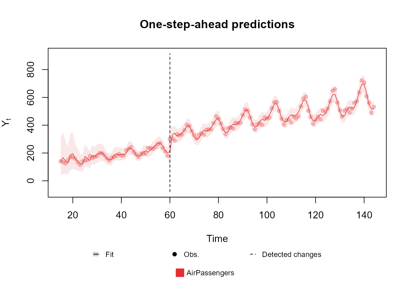

The approach used for automated monitoring is almost identical to that of West and Harrison (1997), chapter 11.4, using Bayes’ factor, such that p.monit\(=0.05\) yields a threshold equivalent to that recommended in West and Harrison (1997).

Tools for sensitivity analysis

In some situations, the user may not be sure about which value to use for some hyperparameter of the model (such as the discount factor or the order of a block) or about the inclusion of some structural block. As such, one might choose to perform a sensitivity analysis on the effect of those choices.

As an motivational example, let us assume that we are unsure about which value to choose for the discount factor in a polynomial trend block of a Poisson model. First, when defining the model structure, we must set the discount factor as a string, which will be used as the label for the unspecified parameter:

level <- polynomial_block(rate = 1, order = 2, D = "D1")

By setting the discount factor as a string, the structural block becomes partially :

summary(level)

Basic DLM block.
latent states: 
    Var.Poly: Level, Slope (2 variable(s))

Linear predictors: 
    rate

Status: undefined
Serie length: 1
Interventions at: 
Number of latent states: 2
Number of linear predictors: 1

As such, this block be used in the fit_model function, unless the value of D1 is specified:

# D1 is missing
season <- harmonic_block(rate = 1, order = 2, period = 12, D = 0.975)
outcome <- Poisson(lambda = "rate", data = c(AirPassengers))
fitted.model <- fit_model(level, season, AirPassengers = outcome)

Error in fit_model(level, season, AirPassengers = outcome): Error: No model to test. Verify if the hyper-parameters are properly specified and if a valid value for condition argument is being passed.

# D1 is set within the fit method
season <- harmonic_block(rate = 1, order = 2, period = 12, D = 0.975)
outcome <- Poisson(lambda = "rate", data = c(AirPassengers))
fitted.model <- fit_model(level, season, AirPassengers = outcome, D1 = 0.95)

As the user can see in the error message above, an undefined dlm_block can only be used to fit a model, unless the value of the missing hyper-parameters are passed as named arguments. Addionally, the user may pass several sequence of values for the missing hyper-parameter. In this case, the fit_model function is used to fit a set of models, while computing some comparative metrics.

fit.dlm_block(...,
  smooth = TRUE, p.monit = NA,
  condition = "TRUE", metric = "log.like",
  pred.cred = 0.95, metric.cutoff = NA, lag = 1
)

The argumetns ..., smooth and p.monit were discussed in Subsection Filtering and smoothing.

Beyond dlm_blocks and dlm_distr objects, the ... argument also must containing, for each undefined parameter (if any exist), the values to be tested. By default, this function will test all possible combinations of the undefined parameter. If the user wishes to skip some combinations, the condition argument can be used to provide a string with the criterion to determine which combinations shall be evaluated.

The remaining options provide some control over the comparative metrics. The metric argument ('mase', 'log.like' or 'interval.score') indicates which metric to use when selecting the best model (all metrics are calculated, not matter the value of the metric argument, but only the best model by the chosen metric is saved). The lag argument indicates the number of steps ahead to be used for predictions (\(0\) indicates filtered predictions and negative values indicate smoothed predictions). The pred.cred argument indicates the credibility of the intervals used when computing the Interval Score. The metric.cutoff argument indicates the number of initial observations to be ignored when computing the metrics.

After evaluating all valid combinations of hyper parameters, the fit_model function returns the best model by the chosen metric, along with a data frame containing the metrics for each model evaluated.

level <- polynomial_block(rate = 1, order = 2, D = "D.level")
season <- harmonic_block(
  rate = "sazo.effect", period = 12,
  order = 2, D = "D.sazo"
)

outcome <- Poisson(lambda = "rate", data = c(AirPassengers))

fit_model(level, season, outcome,
  sazo.effect = c(0, 1),
  D.level = seq(0.8, 1, l = 11),
  D.sazo = seq(0.95, 1, l = 11),
  condition = "sazo.effect==1 | D.sazo==1"
)$search.data |> head()

It is important to note that not all hyper parameters can be tested directly by the fit_model function, indeed, only the components associated with \(F_t\), \(D_t\), \(h_t\), \(H_t\), \(a_1\) and \(R_1\) can be treated as undefined. Still, if the user wants to test some other hyper parameter that cannot be tested directly (such as the order of a polynomial block or the period of a harmonic block), he can create one block for each option and perform a sensitivity analysis for the inclusion/exclusion of each block:

# Creating a block for each order
level <- polynomial_block(rate = "pol.ord.1", order = 1, D = 0.95) +
  polynomial_block(rate = "pol.ord.2", order = 2, D = 0.95) +
  polynomial_block(rate = "pol.ord.3", order = 3, D = 0.95) +
  polynomial_block(rate = "pol.ord.4", order = 4, D = 0.95)
season <- harmonic_block(rate = 1, order = 2, period = 12, D = 0.975)

outcome <- Poisson(lambda = "rate", data = c(AirPassengers))

fit_model(level, season, outcome,
  # Each block can be present (1) or absent (0).
  pol.ord.1 = c(0, 1), pol.ord.2 = c(0, 1),
  pol.ord.3 = c(0, 1), pol.ord.4 = c(0, 1),
  condition = "pol.ord.1+pol.ord.2+pol.ord.3+pol.ord.4==1"
  # Only test combinations with exactly one polynomial block.
)$search.data |> head()

Sampling and hyper parameter estimation

Lastly, one may also want to draw samples from the latent states, linear predictors and/or the parameters \(\eta_t\) of the observational model. This can be useful to evaluate non-linear functions of the model parameters or when the DGLM is only a part of a bigger model, from which the parameters are being estimated with Gibbs Algorithm. It is important to note that, with the method proposed in Alves et al. (2024), sampling from the posterior distribution of the latent states is straight forward, allowing the user to obtain large independent (not approximately independent, but exactly independent) samples with very low computational cost. See West and Harrison (1997), chapter 15, for details about the sampling algorithm.

The kDGLM package offers the simulate function, which provides a routine for drawing independent samples from any fitted model:

simulate(fitted.model, 5000)

For the example above, where our model has \(6\) latent states and \(144\) observations (which yields a total of \(864\) parameters), it takes approximately \(0.3\) seconds to draw a sample of size \(5.000\).

Another useful feature of the kDGLM package is that it provides an approximate value for the Model likelihood \(f(y)= \int_{\mathbb{R}^{n}}f(y|\theta)f(\theta)d\theta\), where \(y\) represents the values for \(Y_t\) for all \(t\) and \(\theta\) represents the values of \(\theta_t\) for all \(t\). This feature can be used for two main purposes: to compare different models and to evaluate the posterior distribution of hyper parameter.

To compare different models, \(\mathcal{M}_1,...,\mathcal{M}_k\) , one can note that \(f(\mathcal{M}_i|y) \propto f(y|\mathcal{M}_i)f(\mathcal{M}_i)\), where \(f(y|\mathcal{M}_i)= \int_{\mathbb{R}^{n}}f(y|\theta,\mathcal{M}_i)f(\theta|\mathcal{M}_i)d\theta\) is the likelihood of model \(\mathcal{M}_i\) and \(f(\mathcal{M}_i)\) is the prior for model \(\mathcal{M}_i\). To evaluate \(f(y|\mathcal{M}_i)\), one can make use of the coef method, the eval_dlm_norm_const or fit_model functions by setting lag to a negative number (the log likelihood metric will be \(\ln f(y|\mathcal{M}_i)\)). Similarly, if the user wants to obtain the marginal posterior distribution of an hyper parameter \(\tau\), it can observe that \(f(\tau|y) \propto f(y|\tau)f(\tau)\), from which \(f(y|\tau)\) can be evaluated using the coef method, the eval_dlm_norm_const or fit_model functions.

H.range <- seq.int(0, 2, l = 100)
log.like.H <- seq_along(H.range)
log.prior.H <- dlnorm(H.range, 0, 1, log = TRUE)
for (i in seq_along(H.range)) {
  level <- polynomial_block(rate = 1, order = 2, H = H.range[i])
  season <- harmonic_block(rate = 1, order = 2, period = 12, D = 0.975)
  # Using only 10 observations, for the sake of a pretty plot. For this particular application, the posterior density of H rapidly becomes highly consentrated in a single value.
  outcome <- Poisson(lambda = "rate", data = c(AirPassengers)[1:10])
  fitted.model <- fit_model(level, season, outcome)
  log.like.H[i] <- eval_dlm_norm_const(fitted.model)
}
log.post.H <- log.prior.H + log.like.H
post.H <- exp(log.post.H - max(log.post.H))
plot(H.range, post.H, type = "l", xlab = "H", ylab = "f(H|y)")

References

Alves, M. B., Migon, H. S., Marotta, R., and dos Santos, S. V., Junior. (2024). K-parametric dynamic generalized linear models: A sequential approach via information geometry.

Bracher, E. L. A. G., Johannes AND Ray. (2021). Evaluating epidemic forecasts in an interval format. PLOS Computational Biology, 17(2), 1–15.

Hyndman, R. J., and Koehler, A. B. (2006). Another look at measures of forecast accuracy. International Journal of Forecasting, 22(4), 679–688.

West, M., and Harrison, J. (1997). Bayesian forecasting and dynamic models (springer series in statistics). Hardcover; Springer-Verlag.

Fitting and analysing models

Table of contents