Creation of model structures

In this section we will discuss the specification of the model structure. We will consider the structure of a model as all the elements that determine the relation between our linear predictor $\vec{\lambda}_t$ and our latent states $\vec{\theta}_t$ though time. Thus, the present section is dedicated to the definition of the following, highlighted equations from a general dynamic generalized model:

$$ \require{color} \begin{equation} \begin{aligned} Y_t|\eta_t &\sim \mathcal{F}\left(\eta_t\right),\\ g(\eta_t) &= {\color{red}\lambda_{t}=F_t'\theta_t,}\\ {\color{red}\theta_t }&{\color{red}=G_t\theta_{t-1}+\omega_t,}\\ {\color{red}\omega_t }&{\color{red}\sim \mathcal{N}_n(h_t,W_t)}. \end{aligned} \end{equation} $$

Namely, we consider that the structure of a model consists of the matrices/vectors $F_t$ , $G_t$ , $\vec{h}_t$ , $H_t$ and $D_t$ .

Although we allow the user to manually define each entry of each of those matrices (which we do not recommend), we also offer tools to simplify this task. Currently, we offer support for the following base structures:

polynomial_block: Structural block for polynomial trends (see West and Harrison, 1997, Chapter 7). As special cases, this block has support for random walks and linear growth models.
harmonic_block: Structural block for seasonal trends using harmonics (see West and Harrison, 1997, Chapter 8).
regression_block: Structural block for (dynamic) regressions (see West and Harrison, 1997, Chapter 6 and 9).
TF_block: Structural block for autoregressive components and transfer functions (see West and Harrison, 1997, Chapter 9 and 13).
noise_block: Structural block for random effects dos Santos et al. (2024).

For the sake of brevity, we will present only the details for the polynomial_block, since all other functions have very similar usage (the full description of each block can be found in the vignette, in the reference manual and in their respective help pages).

Along with the aforementioned functions, we also present some auxiliary functions and operations to help the user manipulate created structural blocks.

In Subsections A structure for polynomial trend models, A structure for dynamic regression models, A structure for harmonic trend models, A structure for autoregresive models and A structure for overdispersed models introduce the several functions design to facilitate the creation of single structural blocks. In those sections we begin by examining simplistic models, characterized by a single structural block and one linear predictor, with a completely known $F_t$ matrix. Subsection Handling multiple structural blocks builds upon these concepts, exploring models that incorporate multiple structural blocks while maintaining a singular linear predictor. The focus shifts in Subsection Handling multiple linear predictors, where we delve into the specification of multiple linear predictors within the same model. In Section Handling unknown components in the planning matrix $F_t$ , the discussion turns to scenarios where $F_t$ includes one or more unknown components. Finally, Subsection Special priors provides a brief examination of functions used to define specialized priors.

A structure for polynomial trend models

polynomial_block(...,
  order = 1, name = "Var.Poly",
  D = 1, h = 0, H = 0,
  a1 = 0, R1 = c(9, rep(1, order - 1)),
  monitoring = c(TRUE, rep(FALSE, order - 1))
)

# When used in a formula
pol(order = 1, D = 0.95, a1 = 0, R1 = 9, name = "Var.Poly")

Recall the notation introduced in Section Notation and revisited at the beginning of this vignette. The polynomial_block function will create a structural block based on West and Harrison (1997), chapter 7. The pol function is a simplified version meant to be used inside formulas in the kdglm function and has the same syntax as the polynomial_block function. This involves the creation of a latent vector $\vec{\theta}_t=(\theta_{1,t},...,\theta_{n,t})'$ , such that:

$\begin{equation} \begin{aligned} \theta_{i,t} &= \theta_{i,t-1}+\theta_{i+1, t-1}+\omega_{i,t}, i=1,...,n-1\\ \theta_{n,t} &= \theta_{n,t-1}+\omega_{n,t},\\ \theta_1&\sim \mathcal{N}_k(a_1,R_1),\\ \omega_{1,t},...,\omega_{n,t}&\sim \mathcal{N}_n(\vec{h}_t,W_t), \end{aligned} \label{eq:defpol} \end{equation}$

where $W_t=Var[\theta_t|\mathcal{D}_{t-1}]\odot (1-D_t) \oslash D_t+H_t$ .

Let’s dissect each component of this specification.

The order argument sets the polynomial block’s order, correlating $n$ with the value passed.

The optional name argument aids in identifying each structural block in post-fitting analysis, such as plotting or result examination (see Section Fitting and analysing models).

The D, h, H, a1, and R1 arguments correspond to $D_t$ , $\vec{h}_t$ , $H_t$ , $\vec{a}_1$ and $R_1$ , respectively.

D specifies the discount matrices over time. Its format varies: a scalar implies a constant discount factor; a vector of size $T$ (the length of the time series) means varying discount factors over time; a $n\times n$ matrix indicates that the same discount matrix is given by D and is the same for all times; a 3D-array of dimension $n\times n\times T$ indicates time-specific discount matrices. Any other shape for D is considered invalid.

h specifies the drift vector over time. If h is a scalar, it is understood that the drift is the same for all variables at all time. If h is a vector of size $T$ , then it is understood that the drift is the same for all variables, but have different values for each time, such that each coordinate $t$ of h represents the drift for time $t$ . If h is a $n \times T$ matrix, then we assume that the drift vector at time $t$ is given by h[,t]. Any other shape for h is considered invalid.

The argument H follows the same syntax as D, since the matrix $H_t$ has the same shape as $D_t$ .

The argument a1 and R1 are used to define, respectively the mean and the covariance matrix for the prior for $\theta_1$ . If a1 is a scalar, it is understood that all latent states associated with this block have the same prior mean; if a1 is a vector of size $n$ , then it is understood that the prior mean $a_1$ is given by a1. If R1 is a scalar, it is understood that the latent states have independent priors with the same variance (this does not imply that they will have independent posteriors); if R1 is a vector of size $n$ , it is understood that the latent states have independent priors and that the prior variance for the $\theta_{i,1}$ is given by R1[i]; if R1 is a $n \times n$ matrix, it is understood that $R_1$ is given by R1. Any other shape for a1 or R1 are considered invalid.

The arguments D, h, H, a1, and R1 can accept character values, indicating that certain parameters are not fully defined. In such cases, the dimensions of these arguments are interpreted in the same manner as their numerical counterparts. For instance, if D is a single character, it implies a uniform, yet unspecified, discount factor across all variables and time points, with D serving as a placeholder label. Should D be a vector of length $T$ (the time series length), it suggests varying discount factors over time, with each character entry in the vector (e.g., D[i]) acting as a label for the discount factor at the respective time point. This logic extends to the other arguments and their various dimensional forms. It’s crucial to recognize that if these arguments are specified as labels rather than explicit values, the corresponding model block is treated as “undefined,” indicating the absence of a key hyperparameter. Consequently, a model with an undefined block cannot be fitted. Users must either employ the specify.dlm_block method to replace labels with concrete values or pass the value of the value of those hyper-parameter as named values to the fit_model function to systematically evaluate models with different values for these labels. Section Tools for sensitivity analysis elaborates on the available tools for sensitivity analysis. Further information about both specify and fit_model is available in the reference manual or through the help function.

Notice that the user does not need to specify the matrix $G_t$ , since it is implicitly determined by the equation and the order of the polynomial block. Each type of block will define it own matrix $G_t$ , as such, the user does not need to worry about $G_t$ , except in very specific circumstances, where an advanced user may need a type of model that is not yet implemented.

The argument ... is used to specify the matrix $F_t$ (see details in Subsection Handling multiple linear predictors). Specifically, the user must provide a list of named values which are arbitrary labels to each linear predictor $\lambda_{i,t}$ , $i=1,\ldots,k$ , and its associated value represents the effect of the level $\theta_{1,t}$ (see Eq. ) in this predictor.

For example, consider a polynomial block of order $2$ , representing a linear growth. If the user passes an extra argument lambda (the naming is arbitrary) as $1$ , then the matrix $F_t$ is created as:

$F_t=\begin{bmatrix}1\\0\end{bmatrix}$

Note that, as the polynomial block has order $2$ , it has $2$ latent states, $\theta_{1,t}$ and $\theta_{2,t}$ . While $\theta_{2,t}$ does not affect the linear predictor lambda directly, it serves as an auxiliary variable to induce a more complex dynamic for $\theta_{1,t}$ . Indeed, by Equation , we have that a second order polynomial block have the following temporal evolution:

$\begin{aligned} \theta_{1,t} &= \theta_{1,t-1}+\theta_{2, t-1}+\omega_{1,t}\\ \theta_{2,t} &= \theta_{2,t-1}+\omega_{2,t},\\ \omega_{1,t},\omega_{2,t}&\sim \mathcal{N}_2(\vec{h}_t,W_t). \end{aligned}$

As such, $\theta_{2,t}$ represents a growth factor that is added in $\theta_{1,t}$ and smoothly changes overtime. Even more complex structures can be defined, either by a higher order polynomial block or by one of the several other types of block offered by the kDGLM.

The specification of values associated to each predictor label is further illustrated in the examples further exhibited in this section.

Lastly, the argument monitoring shall be explained later, in Subsection Intervention and monitoring, which discusses automated monitoring and interventions.

To exemplify the usage of this function, let us assume that we have a simple Normal model with known variance $\sigma^2$ , in which $\eta$ is the mean parameter and the link function $g$ is such that $g(\eta)=\eta$ . Let us also assume that the mean is constant over time and we have no explanatory variables, so that our model can be simply written as:

$$ \begin{aligned} Y_t|\theta_t &\sim \mathcal{N}_1\left(\eta_t, \sigma^2\right),\\ \eta_t &={\color{red}\lambda_{t}=\theta_t,}\\ {\color{red}\theta_t} &{\color{red}=\theta_{t-1}=\theta.} \end{aligned} $$

In this case, we have $F_t=1$ , $G_t=1$ , $D_t=1$ , $h_t=0$ and $H_t=0$ , for all $t$ . Assuming a prior distribution $\mathcal{N}(0,9)$ for $\theta$ , we can create the highlighted structure using the following code:

mean_block <- polynomial_block(eta = 1, order = 1, name = "Mean")

Setting eta=1, we specify that there is a linear predictor named eta, and that $eta = 1 \times \theta$ . Setting order = 1, we specify that $\theta_t$ is a scalar and that $G_t=1$ . We can omit the values of a1 , R1, D, h and H, since the default values reflect the specified model. We could also omit the argument order, since the default is $1$ , but we chose to explicit define it so as to emphasize its usage. The argument name specifies a label for the created block; in this case, we chose to call it “Mean”, to help identify its role in our model.

Suppose now that we have an explanatory variable $X$ that we would like to introduce in our model to help explain the behavior of $\eta_t$ . We could similarly define such structure by creating an additional block such as:

polynomial_block(eta = X, name = "Var X")

By setting eta=X, we specify that there is a linear predictor called eta, and that $eta = X \times \theta$ . If $X=(X_1,...,X_T)'$ is a vector, then we would have $F_t=X_t$ , for each $t$ , such that $eta_t = X_t \times \theta$ .

It should be noted that kDGLM has a specific structural block designed for regressions, regression_block, but we also allow any structural block to be used for a regression, by just setting the value assigned to the predictor equal to the regressor vector $X_t, t=1, \ldots, X_T$ .

The user can specify complex temporal dynamics for the effects of any co-variate. For instance, it could be assumed that a regressor has a seasonal effect on a linear predictor. This this could be accommodated by the insertion of the values of the regressor associated to a seasonal block. The use of seasonal blocks is illustrated in Section Space-time model hospital admissions from gastroenteritis.

So far, we have only discussed the creation of static latent effects, but the inclusion of stochastic temporal dynamics is very straightforward. One must simply specify the values of H to be greater than $0$ and/or the values of D to be lesser than $1$ :

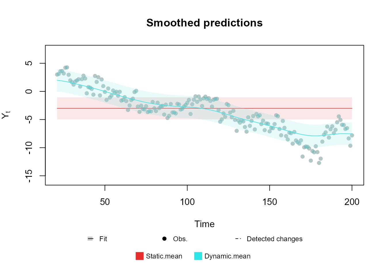
mean_block <- polynomial_block(eta = 1, order = 1, name = "Mean", D = 0.95)

Notice that a dynamic regression model could be obtained by assigning eta=X in the previous code line. Bellow we present a plot of two simple trend models fitted to the same data: one with a static mean and another using a dynamic mean.

In the following example we use the functions Normal, fit_model and the plot method. We advise the reader to initially concentrate solely on the application of the polynomial_block. The functionalities and detailed usage of the other functions and methods, Normal, fit_model, and plot, will be explored in later sections, specifically in Sections Creating the model outcome: and Fitting and analysing models:. The inclusion of these functions in the current example is primarily to offer a comprehensive and operational code sample.

For an extensive presentation and thorough discussion of the theoretical aspects underlying the structure highlighted in this section, interested readers are encouraged to consult West and Harrison (1997), Chapters 6, 7, and 9. Additionally, we strongly recommend that all users refer to the associated documentation for more detailed information. This can be accessed by using the help(polynomial_block) function or consulting the reference manual.

A structure for dynamic regression models

regression_block(...,
  max.lag = 0,
  zero.fill = TRUE,
  name = "Var.Reg",
  D = 1,
  h = 0,
  H = 0,
  a1 = 0,
  R1 = 9,
  monitoring = rep(FALSE, max.lag + 1)
)

# When used in a formula
reg(X, max.lag = 0, zero.fill = TRUE, D = 0.95, a1 = 0, R1 = 9, name = "Var.Reg")

The regression_block function creates a structural block for a dynamic regression with covariate $X_t$ , as specified in West and Harrison (1997), chapter 9. The reg function is a simplified version meant to be used inside formulas in the kdglm function and has the same syntax as the regression_block function. When max.lag is equal to $0$ , this function can be see as a wrapper for the polynomial_block function with order equal to $1$ . When max.lag is greater or equal to $1$ , the regression_block function is equivalent to the superposition of several polynomial_block functions with order equal to $1$ . Specifically, if the linear predictor $\lambda_t$ is associated with this block, we can describe its structure with the following equations:

$\begin{equation} \begin{aligned} \lambda_t&=\sum_{i=0}^{max.lag}X_{t-i}\theta_{i,t},\\ \theta_{i,t}&=\theta_{i,t-1}+\omega_{i,t},\quad \forall i,\\ \omega_{0,t},...,\omega_{max.lag,t}&\sim \mathcal{N}_{max.lag+1}(0,W_t),\\ \theta_{0,1},..., \theta_{max.lag,1}&\sim \mathcal{N}_{max.lag+1}(a_1,R_1), \end{aligned} \end{equation}$ where $W_t=Var[\theta_t|\mathcal{D}_{t-1}]\odot (1-D_t) \oslash D_t+H_t$ .

The usage of the regression_block function is quite similar to that of the polynomial_block function, the only differences being in the max.lag and zero.fill arguments. The max.lag defines the maximum lag of the variable $X_t$ that has effect on the linear predictor. For example, if we define max.lag as $3$ , we would be defining that $X_t$ , $X_{t-1}$ , $X_{t-2}$ and $X_{t-3}$ all have an effect on $\lambda_t$ , such that $max.lag+1$ latent variables are created, each one representing the effect of a lagged value of $X_t$ .

Lastly, the zero.fill argument defines if the package should take the value of $X_t$ to be $0$ when $t$ is non-positive, i.e., if TRUE (default), the package considers $X_t=0$ , for $t=0,-1,...,-max.lag+1$ . If zero.fill is FALSE, then the user must provide the values of $X_t$ as a vector of size $T+max.lag$ (instead of $T$ ), where $T$ is the length of the time series that is being modeled, and the first $max.lag$ values of that vector will be taken as $X_{-max.lag+1},...,X_0$ .

The usage of the remaining arguments is identical to that of the polynomial_block function, and can also be inferred by the previous equation.

Here we present the code for fitting the following model:

$\begin{equation} \begin{aligned} Y_t|\theta_t &\sim Poisson\left(\eta_t\right),\\ \ln(\eta_t) &=\lambda_{t}=X_t\theta_t,\\ \theta_t&=\theta_{t-1}+\omega_t,\\ \omega_t &\sim \mathcal{N}_1(0,W_t), \end{aligned} \end{equation}$ where $X_t$ is a known covariate and $W_t$ is specified using a discount factor of $0.95$ .

regression <- regression_block(The_name_of_the_linear_predictor = X, D = 0.95)

outcome <- Poisson(lambda = "The_name_of_the_linear_predictor", data = data)

fitted.data <- fit_model(regression, outcome)

The detailed theory behind the structure discussed in this section can be found in chapters 6 and 9 from West and Harrison (1997).

A structure for harmonic trend models

harmonic_block(
  ...,
  period,
  order = 1,
  name = "Var.Sazo",
  D = 1,
  h = 0,
  H = 0,
  a1 = 0,
  R1 = 4,
  monitoring = rep(FALSE, order * 2)
)

# When used in a formula
har(period, order = 1, D = 0.98, a1 = 0, R1 = 4, name = "Var.Sazo")

This function will creates a structural block based on West and Harrison (1997), chapter 8, i.e., it creates a latent vector $\theta_t=(\theta_{1,t},\theta_{2,t},...,\theta_{2\times order-1,t},\theta_{2\times order,t})'$ , so that:

$\begin{equation} \begin{aligned} \begin{bmatrix}\theta_{2i -1,t}\\ \theta_{2i,t}\end{bmatrix} = \begin{bmatrix}cos(iw) & sin(iw)\\ -sin(iw) & cos(iw)\end{bmatrix}&\begin{bmatrix}\theta_{2i -1,t-1}\\ \theta_{2i,t-1}\end{bmatrix}+\begin{bmatrix}\omega_{2i -1,t}\\ \omega_{2i,t}\end{bmatrix}, i=1,...,order\\ \theta_{1,1},...,\theta_{2 \times order,1}&\sim \mathcal{N}_{2\times order}(a_1,R_1),\\ \omega_{1,t},...,\omega_{2 \times order,t}&\sim \mathcal{N}_{2\times order}(0,W_t),\\ \end{aligned} \end{equation}$ where $W_t=Var[\theta_t|\mathcal{D}_{t-1}]\odot (1-D_t) \oslash D_t+H_t$ and $w=\frac{2\pi}{period}$ .

Notice that the user does not need to specify the matrix $G_t$ , since it is implicitly determined by the order and the period of the harmonic block, being a block diagonal matrix where each block is a rotation matrix for an angle multiple of $w$ , such that, if period is an integer, $G_t^{period}=I$ . Notice that, when period is an integer, it represents the length of the seasonal cycle. For instance, if we have a time series with monthly observations and we believe this series to have an annual pattern, then we would set the period for the harmonic block to be equal to $12$ (the number of observations until the cycle “resets”). For details about the order of the harmonic block and the representation of seasonal patterns with Fourier Series, see West and Harrison (1997), chapter 8.

The natural usage of this block is for specifying harmonic trends for the model, but it can also be used for explanatory variables with seasonal effect on the linear predictor, for that, see the usage of the regression_block and polynomial_block functions.

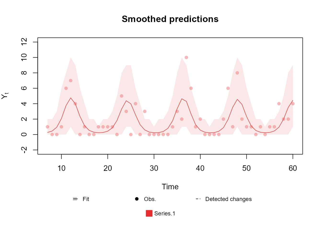
Here we present a simply usage example for a harmonic block with period $12$ :

mean_block <- harmonic_block(
  eta = 1,
  period = 12,
  D = 0.975
)

Bellow we present a plot of a Poisson model with such structure:

The detailed theory behind the structure discussed in this section can be found in chapters 6, 8 and 9 from West and Harrison (1997).

A structure for autoregresive models

TF_block(
  ...,
  order,
  noise.var = NULL,
  noise.disc = NULL,
  pulse = 0,
  name = "Var.AR",
  AR.support = "free",
  a1 = 0,
  R1 = 9,
  h = 0,
  monitoring = TRUE,
  D.coef = 1,
  h.coef = 0,
  H.coef = 0,
  a1.coef = c(1, rep(0, order - 1)),
  R1.coef = c(1, rep(0.25, order - 1)),
  monitoring.coef = rep(FALSE, order),
  a1.pulse = 0,
  R1.pulse = 9,
  D.pulse = 1,
  h.pulse = 0,
  H.pulse = 0,
  monitoring.pulse = NA
)

# When used in a formula
TF(X, order = 1, noise.var = NULL, noise.disc = NULL, a1 = 0, R1 = 9, a1.coef = NULL, R1.coef = NULL, a1.pulse = 0, R1.pulse = 4, name = "Var.AR")

# Wrapper for the autoregressive structure
AR(order = 1, noise.var = NULL, noise.disc = NULL, a1 = 0, R1 = 9, a1.coef = NULL, R1.coef = NULL, name = "Var.AR")

This function creates a structural block based on West and Harrison (1997), chapter 9, i.e., it creates a latent state vector $\theta_t$ , an autoregressive (AR) coefficient vector $\phi_t=(\phi_{1,t},...,\phi_{order, t})'$ and a pulse coefficient vector $\rho_t=(\rho_{1,t},...,\rho_{l,t})'$ , where $l$ is the number of pulses (discussed later on) so that:

$\begin{equation} \begin{aligned} \theta_{t} &= \sum_{i=1}^{k}\phi_{i,t}\theta_{t-i}+\sum_{i=1}^{l}\rho_{i,t}X_{i,t}+\omega_{t},\\ \phi_{i,t}&=\phi_{i,t-1}+\omega^{\text{coef}}_{i,t},\\ \rho_{i,t}&=\rho_{i,t-1}+\omega_{i,t}^{pulse},\\ \omega_{t}&\sim \mathcal{N}_1(h_t,W_t),\\ \omega_{t}^{\text{coef}}&\sim \mathcal{N}_k(h_t^{\text{coef}},W_t^{\text{coef}}),\\ \omega_{t}^{pulse}&\sim \mathcal{N}_l(h_t^{pulse},W_t^{pulse}),\\ \theta_1&\sim \mathcal{N}(a_1,R_1),\\ \phi_1&\sim \mathcal{N}_k(a_1^{\text{coef}},R_1^{\text{coef}}),\\ \rho_1&\sim \mathcal{N}_l(a_1^{pulse},R_1^{pulse}). \end{aligned} \end{equation}$ where:

$\begin{equation} \begin{aligned} W_t&=noise.var&+&\frac{(1-noise.disc)}{noise.disc}Var[\theta_t|\mathcal{D}_{t-1}] & & & & ,\\ W_t^{\text{coef}}&=H_t^{\text{coef}}&+&Var[\phi_t|\mathcal{D}_{t-1}] &\odot& (1-D_t^{\text{coef}}) &\oslash& D_t^{\text{coef}},\\ W^{pulse}_t&=H_t^{pulse}&+&Var[\rho_t|\mathcal{D}_{t-1}] &\odot&(1-D_t^{pulse}) &\oslash&D_t^{pulse}, \end{aligned} \end{equation}$ and $X$ , called pulse matrix, is a known $T \times l$ matrix.

Notice that the user does not need to specify the matrix $G_t$ , since it is implicitly determined by the order of the Tranfer Function (TF) block and the equations above, although, as the reader might have noticed, that evolution will always be non-linear. Since the method used to fit models in this package requires a linear evolution, we use the approach described in West and Harrison (1997), chapter 13, to linearize the previous evolution equation. For more details about the usage of autoregressive models and transfer functions in the context of DLM’s, see West and Harrison (1997), chapter 9.

It is easy to understand the meaning of most arguments of the TF_block function based on the previous equations, but some explanation is still needed for the AR.support argument, plus the arguments related with the so called pulse. We do advise all users to consult the associated documentation for more details (see help(TF_block) or the reference manual).

The AR.support is a character string, either "constrained" or "free". If AR.support is "constrained", then the AR coefficients $\phi_t$ will be forced to be on the interval $(-1,1)$ , otherwise, the coefficients will be unrestricted. Beware that, under no restriction on the coefficients, there is no guarantee that the estimated coefficients will imply in a stationary process, furthermore, if the order of the TF block is greater than 1, then the restriction imposed when AR.support is equal to "constrained" does NOT guarantee that the process will be stationary, as such, the user is not allowed to use constrained parameters when the order of the block is greater than $1$ . To constrain $\phi_t$ to the interval $(-1,1)$ , we apply the inverse Fisher transformation, also known as the hyperbolic tangent function.

The pulse matrix $X$ is informed through the argument pulse, with the dimension of $\rho_t$ being implied by the number of columns in $X$ . It is important to notice that the package expects that $X$ will inform the pulse value for each time instance, interpreting each column as a distinct pulse with an associated coordinate of $\rho_t$ .

Note that when the pulse is absent, $X_t=0, \forall t$ , the TF block is equivalent to a autoregressive block.

Finally, we can summarize the usage of the TF_block function as follows:

a1, R1 are the parameter for the prior for the accumulated effects $(\theta_1,...,\theta_{1-order})'$ ;
noise.var, noise.disc and h define the mean and variance of random fluctuations of $\theta_t$ through time;
a1.coef, R1.coef are the parameter for the prior for the coefficients $\phi_1, ...,\phi_{order}$ ;
h.coef, H.coef and D.coef define the mean and variance of random fluctuations of $\phi_t$ through time;
a1.pulse, R1.pulse are the parameter for the prior for the pulse coefficient $\rho_1$ ;
h.pulse, H.pulse and D.pulse define the mean and variance of random fluctuations of $\rho_t$ through time;
pulse is the pulse matrix $X$ ;
AR.support defines the support for the AR coefficients $\phi_t$ .

Bellow we present the code for a simply $AR(1)$ block with $W_t=0.1, \forall t$ :

mean_block <- TF_block(
  eta = 1,
  order = 1,
  noise.var = 0.1
)

Finally we present a plot of a Gamma model with known shape $\alpha=1.5$ and a AR structure for the mean fitted with simulated data. We will refrain to show the code for fitting the model itself, since we will discuss the tools for fitting in a section of its own.

Some comments about autoregressive models in the Normal family

The user may have notice that the autoregressive block described above is a little different from what is most common in the literature. Specifically, we do not assume that the observed data itself ( $Y_t$ ) follows an autoregressive evolution, but instead $\theta_t$ does. This approach is a generalization of the usual autoregressive model, indeed, if we have that $Y_t$ follows an usual AR(k), such that:

$\begin{equation} \begin{aligned} Y_t&=\sum_{i=1}^{k}\phi_{i,t}Y_{t-1}+\epsilon_t,\\ \epsilon_t &\sim \mathcal{N}_1(0,\sigma_t^2), \end{aligned} \end{equation}$ then, this model can also be written as:

$\begin{equation} \begin{aligned} Y_t|\eta_t&\sim \mathcal{N}_1(\eta_t,0),\\ \eta_t=\theta_t&=\sum_{i=1}^{k}\phi_{i,t}\theta_{t-i}+\omega_t,\\ \omega_t &\sim \mathcal{N}_1(0,W_t), \end{aligned} \end{equation}$ such that this model can be described using the TF_block function.

More generally, if we have that $Y_t|\eta_t \sim \mathcal{F}(\eta_t)$ , where $\mathcal{F}$ is a distribution family contained in the exponential family and indexed by $\eta_t$ , then we have that:

$\begin{equation} \begin{aligned} Y_t|\eta_t &\sim \mathcal{F}(\eta_t),\\ g(\eta_t)=\theta_t&=\sum_{i=1}^{k}\phi_{i,t}\theta_{t-i}+\omega_t,\\ \omega_t &\sim \mathcal{N}_1(0,W_t). \end{aligned} \end{equation}$

It is important to note that there is some caveats about the first specification (the usual one) and the more general one presented above. As the reader will see further bellow, we offer, as a particular case, the Normal distribution with both unknown mean and observational variance, where we can specify predictive strucutre for both the mean and the observational variance. In this model, it does matter if the evolution error is associated with the observation equation or the evolution equation (we cannot specify predictive structure for former, but to the latter we can). For such cases, we recommend the use of the regression_block function instead of the TF_block.

Here we present an example of the specification of an AR(k) using the regression_block function for a time series $Y_t$ of length $T$ :

regression_block(
  mu = c(0, Y[-T]),
  max.lag = k
)

In the Advanced Examples section we will provide a wide range of examples, including ones with the aforementioned structures. In particular, we will present the code for some usual (yet different from what we discussed) forms of AR, including the following model:

$\begin{equation} \begin{aligned} Y_t&=\mu_t+\sum_{i=1}^{k}\phi_{i,t}(Y_{t-1}-\mu_{t-1})+\epsilon_t,\\ \epsilon_t &\sim \mathcal{N}_1(0,\sigma_t^2), \end{aligned} \end{equation}$

A structure for overdispersed models

noise_block(..., name = "Noise", D = 0.99, R1 = 1)

# When used in a formula
noise(name = "Noise", D = 0.99, R1 = 0.1, H = 0)

This function will creates a sequence of independent latent variables $\epsilon_1,...,\epsilon_t$ based on the discussions presented in dos Santos et al. (2024), such that:

$\begin{equation} \begin{aligned} \epsilon_{t} &\sim \mathcal{N}(0,\sigma_t^2),\\ \sigma_t^2&=\frac{t-1}{t}D_t\sigma_{t-1}^2+\frac{1}{t}(1-D_t)\mathbb{E}[\epsilon_{t-1}^2|\mathcal{D}_{t-1}],\\ \sigma_1^2&=R_1. \end{aligned} \end{equation}$

Notice that the user do not need to specify the matrix $G_t$ , since it is implicitly determined by the equations above, such that $G_t=0$ for all $t$ .

It is easy to see the correspondence between most of the arguments of the noise_block function and their respective meaning in the block specification, while the remaining ones follow the same usage seen in the previous block functions (see the polynomial_block function).

As the user must have noticed, this block makes no sense on its own, since it has barely any capability of learning patterns. But, we is shown in the next subsection, structural blocks can be combined with each other, such that the noise block would be only one of several other structural blocks in a model.

To exemplify the utility of this structural block, let us assume we want to model the following (simulated) time series of counts:

Since the data is a counting, its natural to propose a Poisson model, such that:

$\begin{equation} \begin{aligned} Y_t|\theta_t &\sim Poisson\left(\eta_t\right),\\ \ln(\eta_t) &=\lambda_{t}=\theta_t,\\ \theta_t&=\theta_{t-1}+\omega_t,\\ \omega_t &\sim \mathcal{N}_1(0,W_t), \end{aligned} \end{equation}$

Bellow we present that model fitted using the kDGLM package:

level <- polynomial_block(
  rate = 1,
  order = 3,
  D = 0.95
)

fitted.data <- fit_model(level,
  "Model 1" = Poisson(lambda = "rate", data = data)
)

plot(fitted.data, lag = 1, plot.pkg = "base")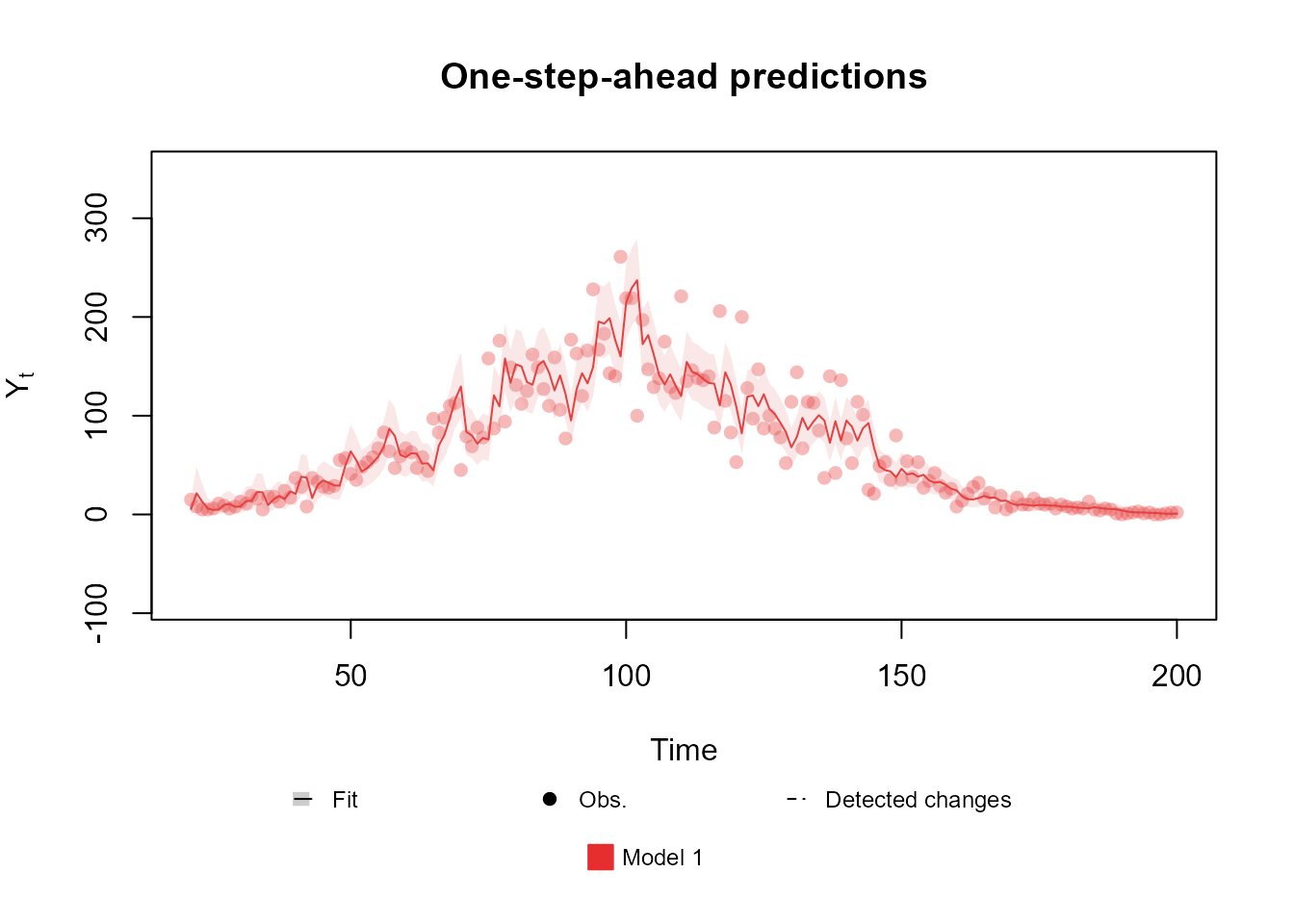

Notice that the data at the middle of the observed period is overdispersed, such that a Poisson model cannot properly address the uncertainty. One could proposed the usage of a Normal model which, indeed, could capture the uncertainty in the middle, but notice that the data at the beginning and at the end of the series has very low values, such that a Normal model would be inappropriate. In such scenario, a better approach would be to add an noise component to the linear predictor, such that it can capture the overdispersion:

level <- polynomial_block(
  mu = 1,
  order = 3,
  D = 0.95
)
noise <- noise_block(
  mu = 1
)

fitted.data <- fit_model(level, noise,
  "Model 2" = Poisson(lambda = "mu", data = data)
)

plot(fitted.data, lag = 1, plot.pkg = "base")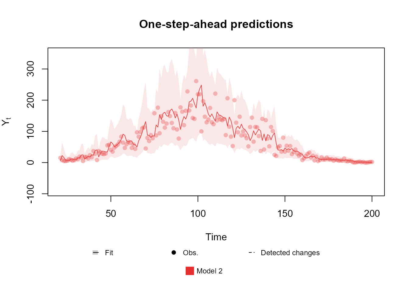

It is relevant to point out that the choice of R1 can affect the final fit, as such, we highly recommend the user to perform a sensibility analysis to help specify the value of R1.

Lastly, as we will see latter on, the noise block can also be useful to model the dependency between multiple time series.

For a more detailed discussion of this type of blocks, see dos Santos et al. (2024).

Handling multiple structural blocks

n the previous subsections, we discussed how to define the structure of a model using the functions polynomial_block, regression_block, harmonic_block, TF_block and noise_block. Each of these functions results in a single structural block. Generally, the user will want to mix multiple types of structures, each one being responsible to explain part of the outcome $Y_t$ . For this task, we introduce an operator designed to combine structural blocks by superposition principle (see West and Harrison, 1997, sec. 6.2), as follows.

Consider the scenario where one wishes to superimpose $p$ structural blocks; for instance: trend, seasonal and regression components ( $p=3$ ). A general overlaid structure is given by the following specifications:

$\begin{aligned} \vec{\theta}_t&=\begin{bmatrix}\vec{\theta}_t^1\\ \vdots\\ \vec{\theta}_t^n\end{bmatrix}, & F_t&=\begin{bmatrix}F_t^1 \\ \vdots \\ F_t^p\end{bmatrix},\\ G_t&=diag\{G_t^{1},...,G_t^{p}\},& W_t&=diag\{W_t^{1},...,W_t^{p}\}, \end{aligned}$

where $diag\{M^1,...,M^{p}\}$ represents a block diagonal matrix such that its diagonal is composed of $M^1,...,M^{p}$ ; $\theta_t$ is the vector obtained by the concatenation of the vectors $\vec{\theta}_t^1,..., \vec{\theta}_t^p$ corresponding to each structural block; and $F_t$ is obtained as follows: if a single linear predictor is considered in the model, $F_t$ is a line vector concatenating $F_t^1,…, F_t^p $. For the case of several predictors ($ k>1$, which will be seen in the next section), the design matrix associated to structural block $i$ , $F_t^i$ , has dimension $n_i k $ and $F_t$ is a $n \times k$ matrix, obtained by the row-wise concatenation of the matrices $F_t^1,..., F_t^p$ , where $n=\sum_{i=1}^p n_i$ .

In this scenario, to facilitate the specification of such model, we could create one structural block for each $\vec{\theta}_t^i$ , $F_t^{i}$ , $G_t^{i}$ and $W_t^{i}$ , $i=1,...p$ , and then “combine” all blocks together. The kDGLM package allows this operation through the function block_superpos or, equivalently, through the + operator:

block_1 <- ...
.
.
.
block_n <- ...

complete_structure <- block_superpos(block_1, ..., block_n)
# or
complete_structure <- block_1 + ... + block_n

For a very high number $p$ of structural blocks, the use of block_superpos is slightly faster. To demonstrate the usage of the + operator, suppose we would like to create a model using four of the structures presented previously (a polynomial trend, a dynamic regression, a harmonic trend and an AR model). We could do so with the following code:

poly_subblock <- polynomial_block(eta = 1, name = "Poly", D = 0.95)

regr_subblock <- regression_block(eta = X, name = "Regr", D = 0.95)

harm_subblock <- harmonic_block(eta = 1, period = 12, name = "Harm")

AR_subblock <- TF_block(eta = 1, order = 1, noise.var = 0.1, name = "AR")

complete_block <- poly_subblock + regr_subblock + harm_subblock + AR_subblock

In the multiple regression context, that is, if more than one regressor should be included in a predictor, the user must specify different regression sub blocks, one for each regressor, and apply the superposition principle to these blocks. Thus, in the previous code lines, X is a vector with $T$ observations of a regressor $X_t$ , already defined in an R object in the current environment and cannot be a matrix of covariates. Ideally, the user should also provide each block with a name to help identify them after the model is fitted, but, if the user does not provide a name, the block will have the default name for that type of block. If different blocks have the same name, an index will be automatically added to the variables with conflicting labels based on the order that the blocks were combined. Note that the automatic naming might make the analysis of the fitted model confusing, specially when dealing with a large number of latent states. With that in mind, we strongly recommend the users to specify an intuitive name for each structural block.

When integrating multiple blocks within a model, it’s crucial to understand how their associated design matrices, denoted as $F_t^{i}$ for each block, are combined. These matrices are concatenated vertically, one below the other. Consequently, since the predictor vector $\vec{\lambda}_t$ is calculated as $F_{t}'\vec{\theta}_t$ , the influence of each block on $\vec{\lambda}_t$ is cumulative. In our previous code example, we introduced a linear predictor named eta. In this context, the operations performed in lines 1, 5, and 7 (corresponding to polynomial_block, regression_block, and TF_block, respectively), are represented as $eta_t=1 \times \theta_{1,t}^{i},i=1,3,4$ ; while in line 3 (corresponding to regression_block), the operation is $eta_t=X_t \times \theta_{1,t}^{2}$ . It’s important to note that each block initially defines eta independently. However, when these blocks are combined, their respective equations are merged. As a result, the complete structure in line 9 can be expressed as:

$eta_t= 1 \times \theta_{1,t}^{1} + X_t \times \theta_{1,t}^{2} + 1 \times \theta_{1,t}^{3} + 1 \times \theta_{1,t}^{4}$

This expression illustrates how the contributions from each individual block are aggregated to form the final model. This methodology allows for the flexible construction of complex models by combining simpler components, each contributing to explain a particular facet of the process $\{Y_t\}_{t=1}^T$ .

Handling multiple linear predictors

As the user may have noticed, more then one argument can be passed in the ... argument. Indeed, if the user does so, several linear predictors will be created in the same block (one for each unique name), all of which are affected by the associated latent state. For instance, take the following code:

polynomial_block(lambda1 = 1, lambda2 = 1, lambda3 = 1) # Common factor

The code above creates $3$ linear predictors $\lambda_{1,t}$ , $\lambda_{2,t}$ and $\lambda_{3,t}$ and a design matrix $F_t=(1,1,1)'$ , such that:

$\begin{aligned} \lambda_{1,t}&=1 \times \theta_{t}\\ \lambda_{2,t}&=1 \times \theta_{t}\\ \lambda_{3,t}&=1 \times \theta_{t} \end{aligned}$

Note that the latent state $\theta_{t}$ is the same for all linear predictors $\lambda_{i,t}$ , i.e., $\theta_{t}$ is a shared effect among those linear predictors which could be used to induce association among predictors. The specification of independent effects to each linear predictor can be done by using different blocks to each latent state:

polynomial_block(lambda1 = 1, order = 1) + # theta_1
  polynomial_block(lambda2 = 1, order = 1) + # theta_2
  polynomial_block(lambda3 = 1, order = 1) # theta_3

When the name of a linear predictor is missing from a particular block, i.e., the name of a linear predictor was passed as an argument in one block, but is absent in another, it is understood that particular block has no effect on the linear predictor that is absent, such that the previous code would be equivalent to:

# Longer version of the previous code for the sake of clarity.
# In general, when a block does not affect a particular linear predictor, that linear predictor should be ommited when creating the block.
polynomial_block(lambda1 = 1, lambda2 = 0, lambda3 = 0, order = 1) + # theta_1
  polynomial_block(lambda1 = 0, lambda2 = 1, lambda3 = 0, order = 1) + # theta_2
  polynomial_block(lambda1 = 0, lambda2 = 0, lambda3 = 1, order = 1) # theta_3

As discussed in the end of Subsection Handling multiple structural blocks, the effect of each block over the linear predictors will be added to each other. As such both codes will create $3$ linear predictors, such that:

$\begin{aligned} \lambda_{1,t}&=1 \times \theta_{1,t} + 0 \times \theta_{2,t} + 0 \times \theta_{3,t}=\theta_{1,t}\\ \lambda_{2,t}&=0 \times \theta_{1,t} + 1 \times \theta_{2,t} + 0 \times \theta_{3,t}=\theta_{2,t}\\ \lambda_{3,t}&=0 \times \theta_{1,t} + 0 \times \theta_{2,t} + 1 \times \theta_{3,t}=\theta_{3,t} \end{aligned}$

Remind the syntax presented in the first illustration of the current section, which guides the creation of common factors among predictors. One can use multiple blocks in the same structure to define linear predictors that share some (but not all) of their components:

polynomial_block(lambda1 = 1, order = 1) + # theta_1
  polynomial_block(lambda2 = 1, order = 1) + # theta_2
  polynomial_block(lambda3 = 1, order = 1) + # theta_3
  polynomial_block(lambda1 = 1, lambda2 = 1, lambda3 = 1, order = 1) # theta_4: Common factor

representing the following structure:

$\begin{aligned} \lambda_{1,t}&=\theta_{1,t}+\theta_{4,t}\\ \lambda_{2,t}&=\theta_{2,t}+\theta_{4,t}\\ \lambda_{3,t}&=\theta_{3,t}+\theta_{4,t}\\ \end{aligned}$

The examples above all have very basic structures, so as to not overwhelm the reader with overly intricate models. Still, the kDGLM package is not limited to in any way by the inclusion of multiple linear predictors, such that any structure one may use with a single predictor can also be used with multiple linear predictors. For example, we could have a model with $3$ linear predictors, each one having a mixture of shared components and exclusive components:

#### Global level with linear growth ####
polynomial_block(lambda1 = 1, lambda2 = 1, lambda3 = 1, D = 0.95, order = 2) +
  #### Local variables for lambda1 ####
  polynomial_block(lambda1 = 1, order = 1) +
  regression_block(lambda1 = X1, max.lag = 3) +
  harmonic_block(lambda1 = 1, period = 12, D = 0.98) +
  #### Local variables for lambda2 ####
  polynomial_block(lambda2 = 1, order = 1) +
  TF_block(lambda2 = 1, pulse = X2, order = 1, noise.disc = 1) +
  harmonic_block(lambda2 = 1, period = 12, D = 0.98, order = 2) +
  #### Local variables for lambda3 ####
  polynomial_block(lambda3 = 1, order = 1) +
  TF_block(lambda3 = 1, order = 2, noise.disc = 0.9) +
  regression_block(lambda3 = X3, D = 0.95)

Now we focus on the replication of structural blocks, for which we apply block_mult function and the associated operator *. This function allows the user to create multiple blocks with identical structure, but each one being associated with a different linear predictor. The usage of this function is as simple as:

base.block <- polynomial_block(eta = 1, name = "Poly", D = 0.95, order = 1)

# final.block <- block_mult(base.block, 4)
# or
# final.block <- base.block * 4
# or
final.block <- 4 * base.block

When replicating blocks, it is understood that each copy of the base block is independent of each other (i.e., they have their own latent states) and each block is associated with a different set of linear predictors. The name of the linear predictors associated with each block are taken to be the original names with an index:

final.block$pred.names

[1] "eta.1" "eta.2" "eta.3" "eta.4"

Naturally, the user might want to rename the linear predictors to a more intuitive label. For such task, we provide the function:

final.block <- block_rename(final.block, c("Matthew", "Mark", "Luke", "John"))
final.block$pred.names

Handling unknown components in the planning matrix $F_t$

In some situations the user may want to fit a model such that:

$\begin{aligned} \lambda_{t}=F_t'\theta_t=\cdots+\phi_t\theta_t +\cdots, \end{aligned}$ in other words, it may be the case that the planning matrix $F_t$ contains one or more unknown components. This idea may be foreign when working with only one linear predictor, but if our observational model has several predictors it could make sense to have shared effects among predictors. Besides, this construction is also natural when modeling multiple time series simultaneously, such as when dealing with correlated outcomes or when working with a compound regression. All those cases will be explored in the Advanced Examples section of the vignette. For now, we will focus on how to specify such structures, whatever their use may be.

For simplicity, let us assume that we want to create a linear predictor $\lambda_t$ such that $\lambda_{t}=\phi_t\theta_t$ . Then the first step would be to create a linear predictor associated with $\phi_t$ (which we will call phi, although the user may call it whatever it pleases the user):

phi_block <- polynomial_block(phi = 1, order = 1)

Notice that we are creating a linear predictor $\phi_t$ and a latent state $\tilde{\theta}_t$ such that $\phi_t=1\times \tilde{\theta}_t$ . Also, it is important to note that the structure for $\phi_t$ could be any other structural block (harmonic, regression, auto regression, etc.).

Now we can create a structural block for $\theta_t$ :

theta_block <- polynomial_block(lambda = "phi", order = 1)

The code above creates a linear predictor $\lambda_t$ and a latent state $\theta_t$ such that $\lambda_t=\phi_t \times \theta_t$ . Notice that the ... argument of any structural block is used to specify the planning matrix $F_t$ , specifically, the user must provide a list of named values, where each name indicates a linear predictor $\lambda_t$ and its associated value represent the effect of $\theta_{t}$ in this predictor. When the user pass a string in ..., it is implicitly that the component of $F_t$ associated with $\theta_t$ is unknown and modeled by the linear predictor labelled as the passed string.

Lastly, as one could guess, it is possible to establish a chain of components in $F_t$ in order to create an even more complex structure. For instance, take the following code:

polynomial_block(eta1 = 1, order = 1) +
  polynomial_block(eta2 = "eta1", order = 1) +
  polynomial_block(eta3 = "eta2", order = 1)

In the first line we create a linear predictor $\eta_{1,t}$ such that $\eta_{1,t}=1 \times \theta_{1,t}$ . In the second line we create another linear predictor $\eta_{2,t}$ such that $\eta_{2,t}=\eta_{1,t} \times \theta_{2,t}=\theta_{1,t} \times \theta_{2,t}$ . Then we create a linear predictor $\eta_{3,t}$ such that $\eta_{3,t}=\eta_{2,t} \times \theta_{3,t}=\theta_{1,t} \times \theta_{2,t} \times \theta_{3,t}$ .

To fit models with non-linear components in the $F_t$ and/or $G_t$ matrices, we use the Extended Kalman Filter (Kalman, 1960; West and Harrison, 1997).

Special priors

As discussed in Subsection A structure for polynomial trend models, the default prior for the polynomial block—as well as for other blocks—assumes that the latent states are independent with a mean $0$ and a variance of $9$ . Users have the flexibility to modify this prior to any combination of mean vector and covariance matrix, although the latent states of different blocks are always assumed to be independent. It is important to note that this independence applies only to the prior distribution; subsequent updates may induce correlations between the latent states.

While this prior setup may be appropriate for a broad range of applications, there may be instances where a user needs to apply a joint prior for latent states across different blocks. For example, if a similar model has previously been fitted to another dataset, an analyst might wish to integrate information from this prior model into the new fitting. To facilitate the specification of a joint prior for any set of latent states, the kDGLM package offers the joint_prior function:

joint_prior(block, var.index = 1:block$n, a1 = block$a1[var.index], R1 = block$R1[var.index, var.index])

The joint_prior function accepts a dlm_block object and returns the same object with a modified prior.

The block argument is a dlm_block object. The syntax of this function is designed to facilitate the use of the pipe operator (either |> or %>%), allowing for seamless integration into piped sequences. For example:

polynomial_block(mu = 1, order = 2, D = 0.95) |>
  block_mult(5) |>
  joint_prior(a1 = prior.mean, R1 = prior.var)
# assuming the objects prior.mean and prior.var are defined.

The var.index argument is optional and indicates the indexes of the latent states for which the prior distribution will be modified.

The a1 and R1 arguments represent, respectively, the mean vector and the covariance matrix for the latent states that the user wishes to modify the prior for.

The user may also want to specify some special priors that impose a certain structure for the data. For instance, the user may believe that a certain set of latent state sum to $0$ or that there is a spacial structure to them. This is specially relevant when modelling multiple time series, for instance, lets say that we have $r$ series $Y_{i,t}$ , $i=1,...r$ , such that:

$\begin{aligned} Y_{i,t}|\eta_{i,t} &\sim Poisson(\eta_{i,t})\\ \ln(\eta_{i,t})&=\lambda_{it}=\mu_t+\alpha_{i,t},\\ \sum_{i=1}^{r} \alpha_{i,t}&=0, \forall t. \end{aligned}$

Similarly, one could want to specify a CAR prior (Banerjee et al., 2014; Schmidt and Nobre, 2018) for the variables $\alpha_1,...\alpha_r$ , if the user believes there is spacial autocorrelation.

For these scenarios, the kDGLM package provides functions to facilitate the specification of special priors for structural blocks, such as the zero_sum_prior and the CAR_prior. Their general usage is analogous to the joint_prior function. Details on these functions will be omitted in this document for the sake of brevity. For comprehensive usage instructions, please refer to the vignette or the associated documentation.

References

Banerjee, S., Carlin, B. P., and Gelfand, A. E. (2014). Hierarchical modeling and analysis for spatial data. Chapman; Hall/CRC.

dos Santos, S. V., Junior, Alves, M. B., and Migon, H. S. (2024). An efficient sequential approach for joint modelling of multiple time series.

Kalman, R. E. (1960). A new approach to linear filtering and prediction problems. Transactions of the ASME–Journal of Basic Engineering, 82(Series D), 35–45.

Schmidt, A. M., and Nobre, W. S. (2018). Conditional autoregressive (CAR) model. In Wiley StatsRef: Statistics reference online, pages 1–11. John Wiley & Sons, Ltd.

West, M., and Harrison, J. (1997). Bayesian forecasting and dynamic models (springer series in statistics). Hardcover; Springer-Verlag.

Creation of model structures

Table of contents